
Figures & data
Figure 1. The location of the seven ARS watersheds over a generalized landcover data layer.
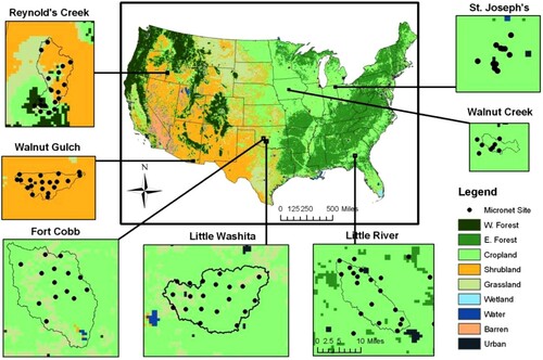
Figure 2. Temporal stability plots of (a) Little River, Georgia and (b) Little Washita, Oklahoma. Error bars denote standard deviations of individual sensors’ reported values. Watershed weighted averages represent the overall watershed average, as determined by sensor positions and its’ associated confidence interval.
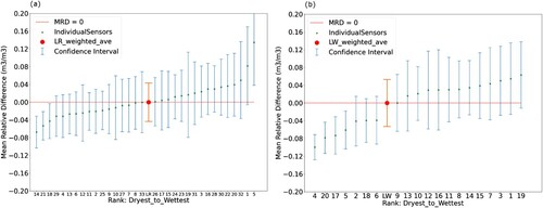
Figure 3. Annual distributions in Reynolds Creek, Idaho. (a) 2004, (b) 2005, and (c) 2006. Error bars denote annual standard deviation of reported sensor values.
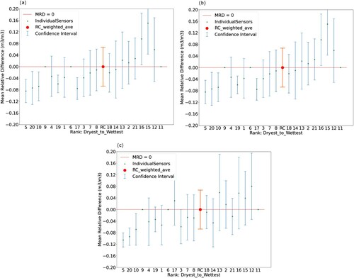
Table 1. Annual rank correlations for each of the ARS watersheds.
Figure 4. Fort Cobb, Oklahoma, sensor distributions by year. (a) Sensor #6, (b) Sensor #7, (c) Sensor #13. Error bars denote annual standard deviation of reported sensor values.
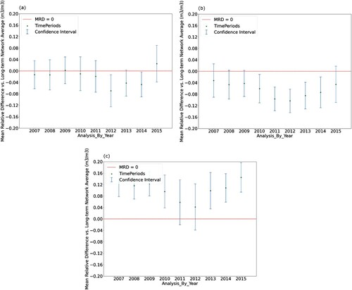
Figure 5. Temporal stability plots for Reynolds Creek, Idaho. (a) May, (b) June, (c) July. Error bars denote monthly standard deviation of reported sensor values.
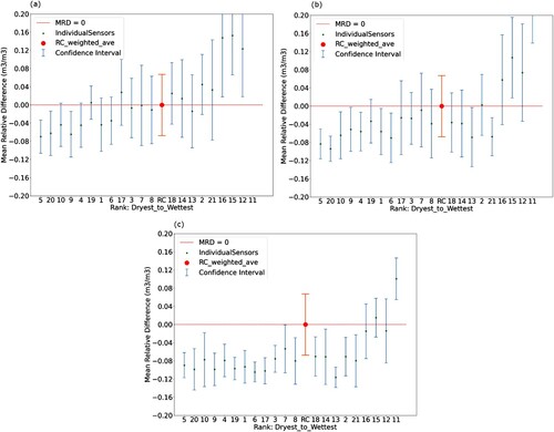
Table 2. Monthly rank correlation for each ‘warm’ month for each watershed.
Figure 6. Walnut Gulch, Arizona, sensor distributions by month. (a) Sensor #18, (b) Sensor #36, (c) Sensor #2. Error bars denote monthly standard deviation of reported sensor values.
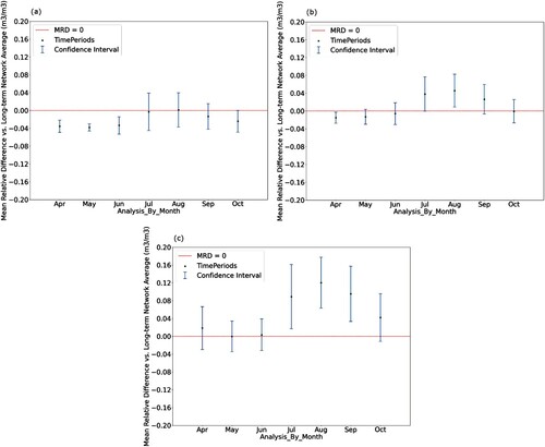
Figure 7. Triple colocation error for an increasing number of sensors at the South Fork, network.
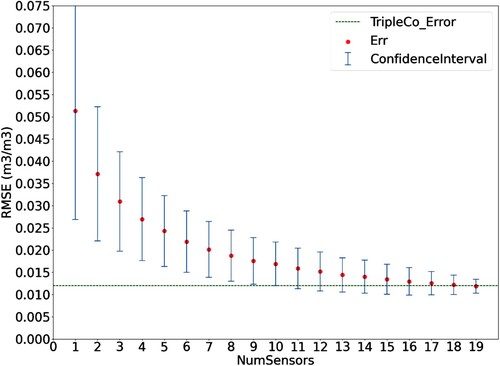
Table 3. Number of sensors needed to estimate full network average for each watershed. Walnut Gulch is not included in this analysis as no timestamp contain all 54 sensors was available.