Figures & data
Figure 1. Overall framework.
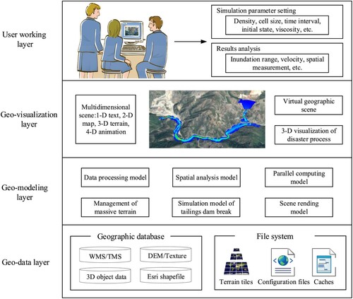
Figure 2. Terrain-sensitive meshing process.
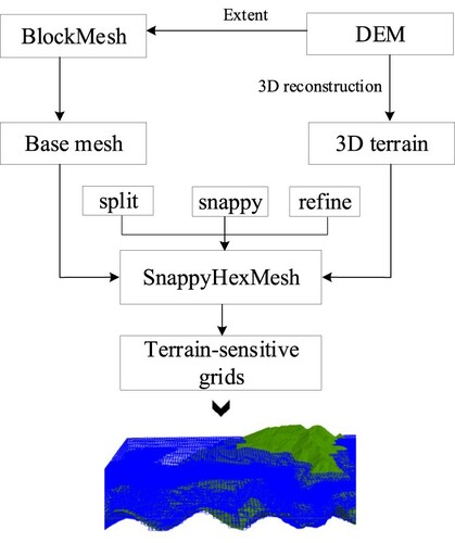
Figure 3. Simulation workflow of dam-break disasters in the virtual geographic environment.
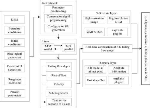
Figure 4. Parameters setting dialog.
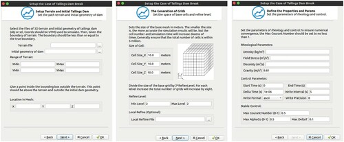
Figure 5. Domain decomposition process.
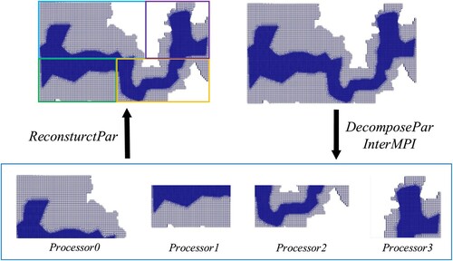
Figure 6. UML sequence diagram of parallel numerical computing in a cluster.
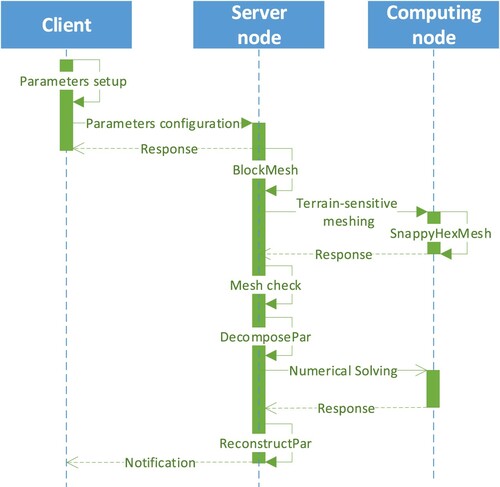
Figure 7. Mesh clipping and different rendering forms of simulation results: (a) diagram of mesh clipping; (b) simulation result rendered in surface form; and (c) simulation result rendered in wireframe form.
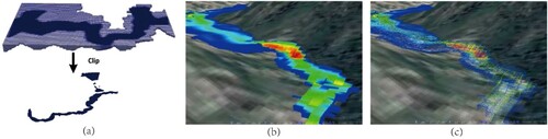
Figure 8. The main interface and some features of the prototype VGE: (a) main interface; (b) spatial annotation and measurement; (c) visibility analysis; and (d) terrain grid generation.
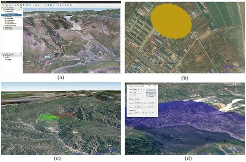
Figure 9. Typical simulated results are visualized in TDBSim. The result is rendered at (a) ; (b)
; (c)
; and (d)
A – location of rail network. B – location of small community. C – location of Parque da Cachoeira. D – location of Paraopeba river. The base map is the satellite image (Sentinel S2). The color map of the simulation results is mapped by velocity characteristics.
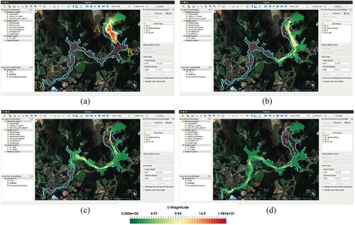
Figure 10. Field investigation photos of the A’xi tailings dam: (a) tailings in the A’xi tailings dam and (b) landforms downstream and environmental protection depot of the tailings dam.
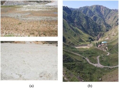
Figure 11. Typical simulated results are visualized in VGE. The result is rendered at (a) ; (b)
; (c)
; and (d)
.
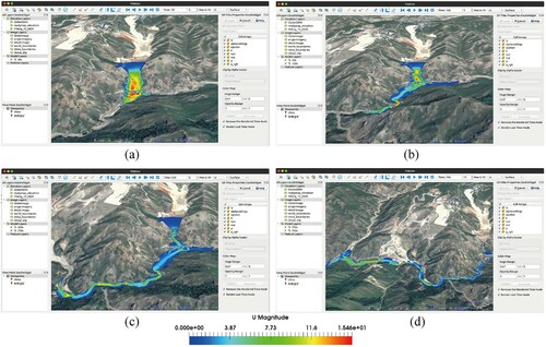
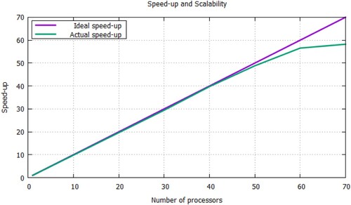
Figure 12. Parallel scalability testing.