An investigation on microwave transmissivity at frequencies of 18.7 and 36.5 GHz for diverse forest types during snow season

Figures & data

Figure 1. Location map of the study area showing the different climate types of the sampling sites. Data source: Resource and Environmental Science and Data Center (http://www.resdc.cn).

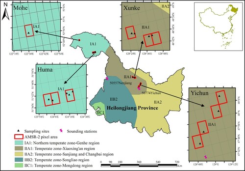
Figure 2. Land cover type of the AMSR-2 pixels where sampling sites locate. Data source: ChinaCover2010, National Earth System Science Data Sharing Infrastructure, National Science & Technology Infrastructure of China (http://www.geodata.cn).

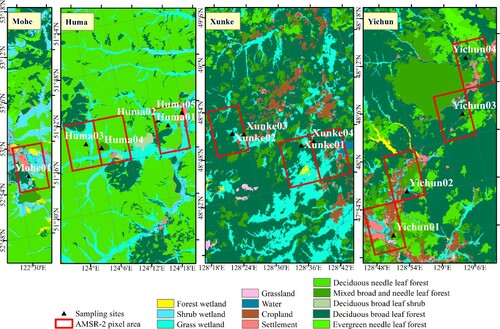
Figure 3. Configuration of the radiometer observations viewed from (a) side and (b) front; and (c) description of the measured T_B from the canopy.

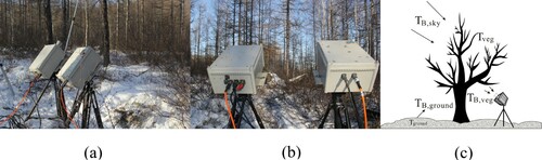
Table 1. Parameters of forest canopies and snow profiles for each tree sample plot.

		Forest characteristic parameters						Snow characteristic parameters
Sample plot	Date of observation	Stand density (trees/ha)	Height (m)	Woody stem volume (m³/ha)	Broad leaf forest (%)	Needle leaf forest (%)	Dominant tree species/forest type	Air temperature (°C)	Snow depth (m)	Snow density (g/cm³)	Effective snow grain diameter (mm)	Snow temperature (°C)
Huma01	2016/12/15	850	12	70	0	100	DNF	–14	0.19	0.131	1.13	–13.5
Huma02	2016/12/16	3316	12.5	153	22	78	DNF	–12	0.19	0.127	1.06	–12.4
Huma03	2016/12/17	1118	10.3	53	4	96	DNF	–5	0.16	0.113	1.06	–9.2
Huma04	2016/12/18	2150	12.6	135	7	93	DNF	–14.5	0.16	0.126	1.16	–12.8
Huma05	2016/12/19	1421	15.5	156	0	100	DNF	–18	0.14	0.145	1.2	–15.8
Mohe01	2016/12/20	3266	10.7	104	75	25	DBF	–19	0.14	0.15	1.23	–12.9
Yichun01	2016/12/23	2500	12	125	36	64	GNF	–18	0.19	0.139	1.3	–11
Yichun02	2016/12/24	2267	15.5	234	0	100	DNF	–16	0.17	0.14	1.28	–12.8
Yichun03	2016/12/25	1704	14	205	12	88	GNF	–13	0.2	0.156	1.39	–10.6
Yichun04	2016/12/26	901	18.4	292	28	72	DNF	–17.5	0.23	0.13	1.38	–12.4
Xunke01	2016/12/27	3209	12.6	153	94	6	DBF	–14.5	0.23	0.157	1.42	–13.3
Xunke02	2016/12/28	1592	10	100	93	7	DBF	–16	0.21	0.141	1.41	–10.8
Xunke03	2016/12/29	2821	9.4	98	93	7	DBF	–15	0.21	0.148	1.45	–11.6
Xunke04	2016/12/29	1078	9.3	28	100	0	DBF	–16	0.25	0.155	1.42	–11.3

Table 2. Average experimental form factor $\left(f_{∍}\right)$ of the main tree species in China

Form factor level	Tree species	Experimental form factor	Applicable tree species
I	Coniferous tree	0.45	Yunnan pine, fir and general strong shade-tolerant coniferous species
II		0.43	Seeding Chinese fir, spruce and general shade-tolerant coniferous species
III		0.42	Chinese fir (regardless of origin), Korean pine, Huashan pine, Huangshan pine and general neutral coniferous species
IV		0.41	Plugged fir, Tianshan spruce, willow fir, Xingan larch, Xinjiang larch, camphor pine, red pine, black pine, oil pine and general light-loving coniferous species
V	Broad-leaved tree	0.40	Poplar, birch, willow, linden, ash, Mongolian oak, oak, cycad, acacia, elm, camphor, eucalyptus and other general broadleaf species, mixed broadleaf forests in Hainan, Yunnan, etc.
VI	Coniferous tree	0.39	Masson pine and general strong light-loving coniferous species

Figure 4. Composition of tree species and woody stem volume at each tree sample plot.

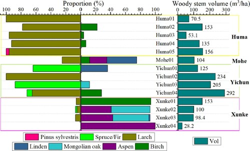
Figure 5. Photos of radiometric measurements corresponding to different forest types.

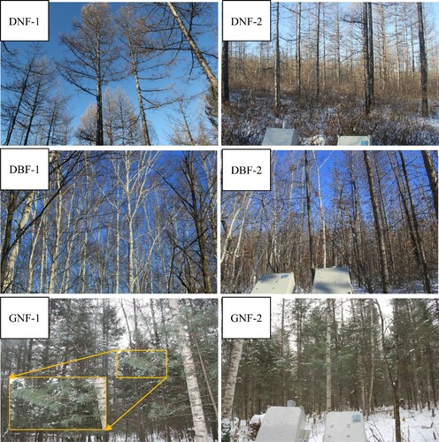
Figure 6. Transmissivity of each tree sample plot at 18.7- and 36.5- GHz, H and V polarizations, at 55° incidence angle, with woody stem volume.

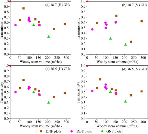
Figure 7. Polarization difference of transmissivity at 18.7 and 36.5 GHz with stand density and woody stem volume.

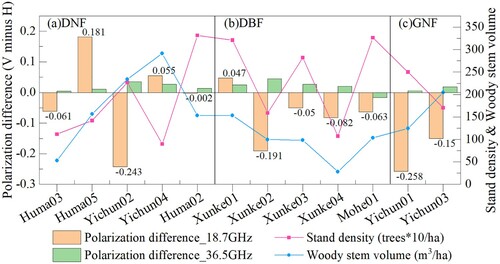
Table 3. Averaged polarization difference in transmissivity for different forest types with stand density and woody stem volume information.

Forest type	Averaged ρ (trees/ha)	Averaged Vol (m³/ha)	Averaged PD (γ(V) – γ(H))
			18.7 GHz	36.5 GHz
DNF	1718	156	–0.01	0.02
DBF	2393	97	–0.07	0.02
GNF	2102	165	–0.20	0.01

Figure 8. Retrieved transmissivity as a function of Vol for different forest types: (a) DNF, (b) DBF and, (c) GNF. The solid lines correspond to the optimized fitting models. Dashed line corresponds to the Kruopis γ model over its validity range (0–150 m³/ha), at 55° incidence angle. Values are referred to the fitted model. The red dots and lines refer to the vertical polarization, and the blue refers to the horizontal polarization.

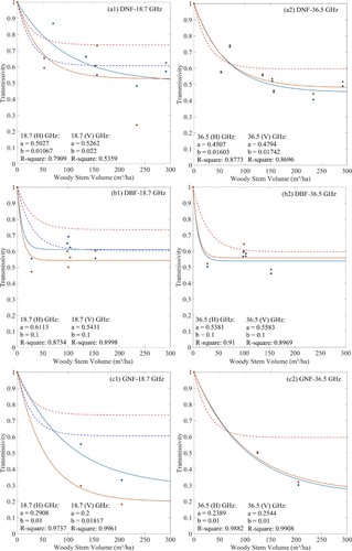
Table 4. Parameters in our γ model for each frequency and polarization at 55° incidence angle retrieved from curve-fitting on the measurements, shown in Figure 7 and compared to Kruopis γ model. (Note that the coefficients a and b in Kruopis γ model were obtained at an incidence angle of 55°.)

Forest Type	Frequency (polarization) GHz	Parameters in Kruopis γ model				Parameters in our γ model
		a	b	γs	Vols	a	b	γs	Vols
DNF	18.7 (H)	0.61	0.035	0.61	119	0.50	0.011	0.50	431
	18.7 (V)	0.74		0.74	102	0.53	0.022	0.53	205
	36.5 (H)	0.60*		0.60	120	0.45	0.016	0.45	300
	36.5 (V)	0.60		0.60	120	0.48	0.017	0.48	269
DBF	18.7 (H)	0.61	0.035	0.61	119	0.61	0.100	0.61	42
	18.7 (V)	0.74		0.74	102	0.54	0.100	0.54	44
	36.5 (H)	0.60*		0.60	120	0.54	0.100	0.54	45
	36.5 (V)	0.60		0.60	120	0.56	0.100	0.56	44
GNF	18.7 (H)	0.61	0.035	0.61	119	0.29	0.010	0.29	550
	18.7 (V)	0.74		0.74	102	0.20	0.018	0.20	330
	36.5 (H)	0.60*		0.60	120	0.24	0.010	0.24	576
	36.5 (V)	0.60		0.60	120	0.25	0.010	0.25	568

Figure 9. Variation of transmissivity retrieved by our γ model against Vol for three forest types at the same frequency and polarization.

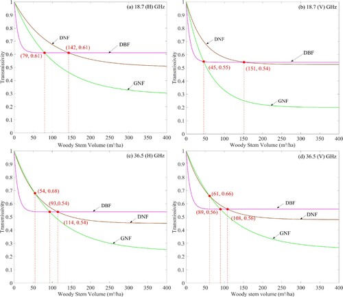
Table 5(a). Comparison of the different transmissivity models with ${\kappa }_{e\mathrm{\_}Hallikainen}$ used to be incorporated into the forward model suite for simulation results against AMSR-2 T_B and the improvement in accuracy.

	Simulation with Kruopis γ model				Simulation with our γ model				Improvement in accuracy (%)
	18.7 (H)	18.7 (V)	36.5 (H)	36.5 (V)	18.7 (H)	18.7 (V)	36.5 (H)	36.5 (V)	18.7 (H)	18.7 (V)	36.5 (H)	36.5 (V)
DNF	6.9	6.3	10.3	7.6	7.1	2.9	7.3	5.8	−2	54	30	25
DBF	4.0	2.0	9.4	9.8	4.0	2.3	9.6	9.9	0	−13	−2	−2
GNF	9.5	7.0	14.3	11.3	8.5	6.3	10.5	8.8	11	10	27	22
Avg.	6.5	5.3	10.7	9.0	6.4	3.4	8.6	7.9	2	36	19	12

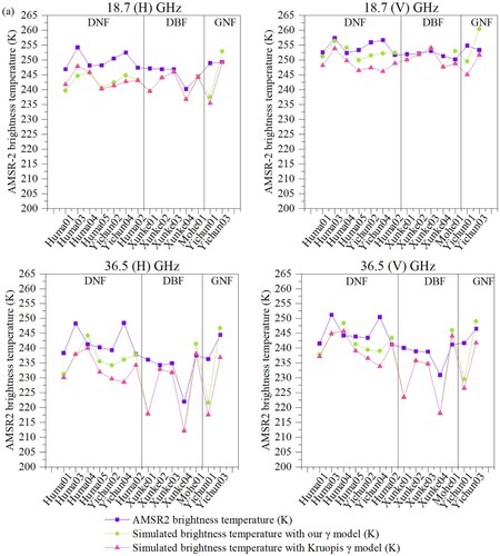
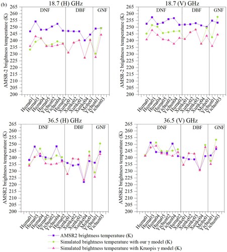
Table 5(b). Same as Table 5(a), except that the extinction coefficients were changed to ${\kappa }_{e\mathrm{\_}Roy}$.

	Simulation with Kruopis γ model				Simulation with our γ model				Improvement in accuracy (%)
	18.7 (H)	18.7 (V)	36.5 (H)	36.5 (V)	18.7 (H)	18.7 (V)	36.5 (H)	36.5 (V)	18.7 (H)	18.7 (V)	36.5 (H)	36.5 (V)
DNF	11.9	12.8	6.4	4.3	12.1	7.2	4.7	4.1	−2	42	26	4
DBF	10.6	9.0	5.1	4.7	10.5	8.5	5.7	5.2	0	6	−12	−10
GNF	15.4	14.8	7.6	4.7	13.2	9.2	6.7	5.6	14	37	12	−20
Avg.	12.0	11.9	6.1	4.5	11.8	8.0	5.4	4.8	2	32	12	−6

Figure 11. $T_{B,veg,\downarrow }$ observed on multiple incidence angles and azimuths at (a) 18.7- and (b) 36.5-GHz, H and V polarizations.

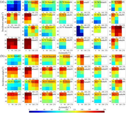
Figure 12. Estimations of the transmissivity with error bars in Case 1 at a fixed incidence angle of 50°: (a) 18.7 GHz and (b) 36.5 GHz; and Case 2 at a unified incidence angle of 55°: (c) 18.7 GHz and (d) 36.5 GHz.

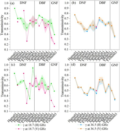
Table 6. Std of $T_{B,veg,\downarrow }$ from all sample plots at multi- azimuth and incidence angles for each frequency and polarization.

Frequency (polarization) GHz	Case 1: Different azimuths at the same incidence angle				Case 2: Different incidence angles at the same azimuth angle
	60°	50°	40°	mean	0°	90°	180°	270°	mean
18.7 (H)	12 ± 10	12 ± 10	14 ± 10	13	20 ± 8	20 ± 8	23 ± 7	10 ± 6	20
18.7 (V)	11 ± 15	9 ± 10	13 ± 11	11	19 ± 9	21 ± 11	19 ± 3	12 ± 8	19
36.5 (H)	8 ± 7	9 ± 7	10 ± 8	9	21 ± 6	20 ± 6	21 ± 7	13 ± 2	20
36.5 (V)	9 ± 8	9 ± 7	10 ± 8	9	20 ± 6	19 ± 6	21 ± 7	12 ± 2	19