Fine scale optical remote sensing experiment of mixed stand over complex terrain (FOREST) in the Genhe Reserve Area: objective, observation and a case study

Figures & data

Figure 1. Multi-scale observations in the FOREST experiment.

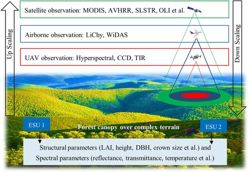
Table 1. Summary of the FOREST experiment composition and measured parameters.

Composition	Instruments	Description	Parameters
Airborne experiments	LiCHy	LiDAR, CCD, hyperspectral integrated system	Digital Surface Model (DSM), Digital Elevation Model (DEM), Canopy Height Model (CHM), Nadir hyperspectral reflectance
	WiDAS	Multi-spectral multi-angle integrated system	Multi-angle Multi-spectral reflectance, Multi-angle brightness temperature
UAV experiments	UAV-CCD	UAV + Sony A7	Reflectance
	UAV-Hyperspectral	UAV + Headwall	Nadir hyperspectral reflectance
	UAV-TIR	UAV + FLIR TAU640	Multi-angle brightness temperature
Ground experiments	Laser rangefinder	For structural parameter	Tree height
	Tape	For structural parameter	DBH, Crown size
	Li-3000	For structural parameter	Leaf size
	Tracing Radiation and Architecture of Canopies (TRAC)	For structural parameter	LAI, CI
	LAISmart	For structural parameter	LAI
	PocketLAI	For structural parameter	LAI
	LAI2000	For structural parameter	LAI, ALIA
	Hemiview	For structural parameter	LAI, ALIA, CI
	Terrestrial LiDAR	For structural parameter	LAI, ALIA, CI
	Nikon D3000	For structural parameter	FVC
	Integrating sphere	For spectral parameter	leaf reflectance
	ASD	For spectral parameter	leaf transmittance, background reflectance, bark reflectance
	FLIR T440	For spectral parameter	leaf temperature, background temperature, bark temperature

Figure 2. Coverage of airborne and UAV observations located in the Genhe Reserve Area.

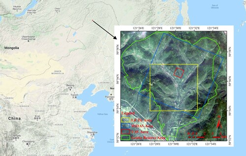
Table 2. Parameters of the LiCHy instruments.

LiDAR: Riegl LMS-Q680i	CCD: DigiCAM-60	Hyperspectral: AISA Eagle II
Wavelength: 1550 nm	Wavelength: RGB	Spectral range: 400–970 nm
Laser beam divergence: 0.5mrad	Pixel resolution: 8956×6708	Spatial pixels: 1024
Laser pulse length: 3 ns	Sensor size: 40.3×53.78 mm^2	Spectral resolution: 3.3 nm
Scan angle range: ±30°	Field of view: 56.2°	Field of View: 37.7
Maximum Laser pulse: 400 KHz	Pixel size: 6 μm	Maximum bands: 488
Maximum scanning speed: 200/s	Radiometric resolution: 16 bits	Recorded Bands: 64
Waveform sampling: 1 ns	Focal length: 50 mm	Focal length: 18.1 mm
Vertical accuracy: 0.15 m	-	Frame rate: 160 frames/s

Figure 3. Estimated KEA DSM from LiCHy-LiDAR measurement (a); estimated KEA DEM from DSM (b); reflectance image of the red band (656 nm) of the KEA obtained by the LiCHy-AISA Eagle II hyperspectral sensor (c); reflectance image of the NIR band (907 nm) of the KEA obtained by the LiCHy-AISA Eagle II hyperspectral sensor (d).

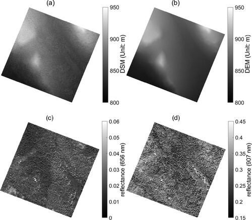
Figure 4. The WiDAS flight tracks (a) and the generated digital orthographic map of the KEA with spatial resolution equal to 0.4 m using Phase iXa 645DF camera (b).

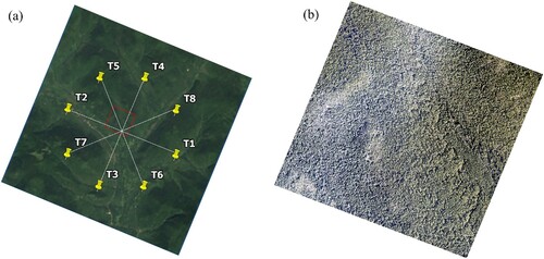
Table 3. Parameters of the WiDAS sensors with a flight height of 2000m.

	iXa 645DF	Condor-MS5	Condor-MS5	FLIR A655sc
Wavelength(nm)	RGB	460,555, 620,685,760	460,555, 620,685,760	7500–14000
Pixels	7760×10328	1360×1024	1360×1024	640×480
FOV	70×87	32×24	32×24	68×54
Oblique Angle	0	14	44	26
Swath (m)	3796	850	850	2038

Figure 5. Flights, sensors and artificial geometric targets of UAV observations.

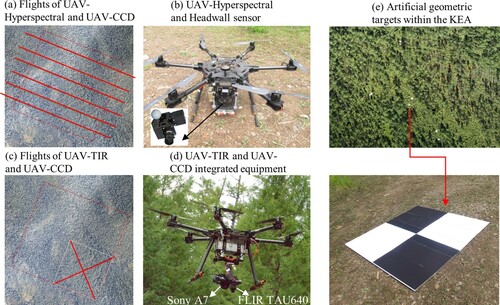
Table 4. Parameters of three UAV sensors.

UAV-CCD	UAV-Hyperspectral	UAV-TIR
Type: Sony A7	Type: Headwall	Type: FLIR TAU640
Wavelength: RGB	Wavelength: 0.38–1.0 μm	Wavelength: 7.5–14 μm
Pixels: 7360×4144	Pixels: 1004×1	Pixels: 640×512
Radiometric resolution: 8 bits	Spectral resolution: 5 nm	Radiometric resolution: 12 bits
Focal length: 35 mm	Focal length: 8 mm	Focal length: 7.5 mm
Weight:0.4 kg	Weight: 0.9 kg	Weight: 0.3 kg
Aim: provide base map	Maximum bands: 325	Pixel size: 17 μm

Figure 6. EVI histogram of the entire KEA (a) and twenty ESUs (b) in the growth stage of 2015, spatial locations (c) and the lateral photos (d) of twenty ESUs.

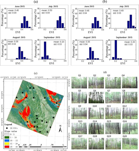
Figure 7. Average height and crown size of pine (a); the scatter plot between the tree height and DBH of pine (b); average height and crown size of birch (c); and the scatter plot between the tree height and DBH of birch (d).

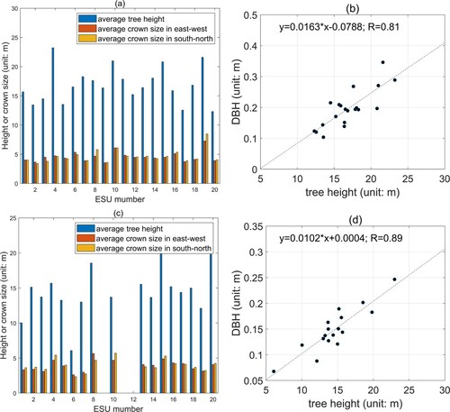
Figure 8. Different sampling approaches for Hemiview (a), LAI-2000 (b), LAISmart (c), PocketLAI (d), and Nikon D3000 camera (e).

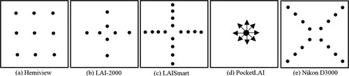
Figure 9. Time series of LAI of all ESUs measured by LAISmart.

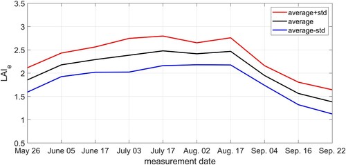
Figure 10. Scatter plot between the in situ-measured FVC and the measured LAIe using LAIsmart in Aug. 02, 2016 (a); and the measured CI using TRAC in ESUs in Aug. 08, 2016 (b).

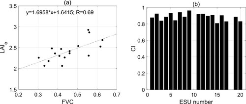
Figure 11. The measured reflectance of pine leaves (a), reflectance of white birch leaves (b), transmittance of white birch leaves (c) and reflectance of background (d). The red, blue, and black line represent the maximum, minimum and average value of the reflectance spectra, respectively.

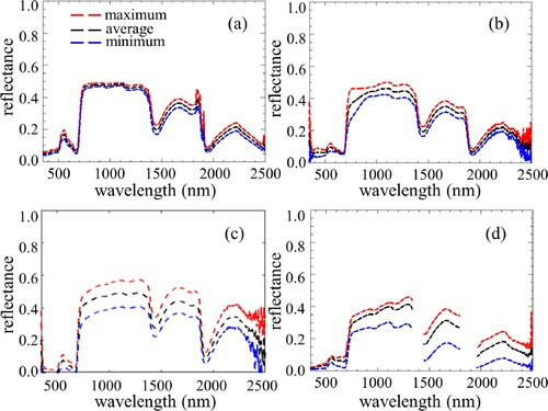
Figure 12. Daytime temperature variation of six components measured on August 19, 2016.

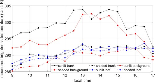
Figure 13. Flowchart of a case study of large-scale canopy reflectance simulation using LESS for the evaluation of the reconstructed 3D scenes based on FOREST dataset.

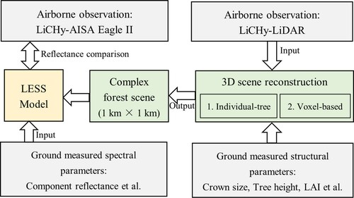
Figure 14. Estimated KEA CHM with spatial resolution of 0.5 m (i.e. DSM-DEM) (a) and KEA PAI with spatial resolution of 2 m from LiCHy-LiDAR (b); pine trees with heights of 7.2, 12.68, 18.42 m, respectively, and birch trees with heights of 13.2, 17.8 and 24.9 m, respectively (c); three typical cells with different amounts of leaves with leaf area volume density (LAVD) of 0.5, 1.5 and 2.5, respectively (d); reconstructed 3D scene using individual-tree approach (e); reconstructed 3D scene using voxel-based approach (f).

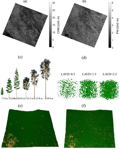
Figure 15. LESS simulated image of the red band (a) and the NIR band (b) using the individual-tree approach; LESS simulated image of the red band (c) and the NIR band (d) using the voxel-based approach; histogram of the reflectance bias of the LESS-simulated image of the red band (e) and the NIR band (f) using the individual-tree approach; histogram of the reflectance bias of the LESS-simulated image of the red band (g) and the NIR band (h) using the voxel-based approach.

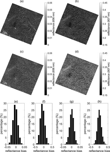
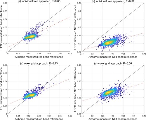
Figure 16. Scatter plot of the LiCHy image and LESS simulated image at 656 nm using the individual-tree approach (a); scatter plot of the LiCHy image and LESS simulated image at 907 nm using the individual-tree approach (b); scatter plot of the LiCHy image and LESS simulated image at 656 nm using the voxel-based approach (c); scatter plot of the LiCHy image and LESS simulated image at 907 nm in the voxel-based approach (d).

Table

FOREST	Fine scale Optical Remote sensing Experiment of mixed Stand over complex Terrain	KEA	Key Experiment Area
ESU	Elementary Sampling Unit	LESS	LargE-Scale remote sensing data and image Simulation framework over heterogeneous 3D scenes
RAMI	RAdiative transfer Model Intercomparison	BOREAS	Boreal Ecosystem-Atmosphere Study
COMPLICATE	Complicate Observations and Multi-Parameter Land Information Constructions on Allied Telemetry Experiment	LiDAR	Light Detection And Ranging
CCD	Charge Coupled Device	DBH	Diameter at Breast Height
PAI	plant area index	LAI	Leaf Area Index
ALIA	Average Leaf Inclination Angle	FVC	Fraction of Vegetation Cover
CI	Clumping Index	LiCHy	LiDAR-CCD-Hyperspectral integrated mission
WiDAS	Wide-angle Infrared Dual-mode line/area Array Scanner	UAV	Unmanned Aerial Vehicle
WATER	Watershed Allied Telemetry Experimental Research	HiWATER	Heihe Watershed Allied Telemetry Experimental Research
BRDF	Bi-directional Reflectance Distribution Function	DBT	Directional Brightness Temperature
TRAC	Tracing Radiation and Architecture of Canopies	DSM	Digital Surface Model
DEM	Digital Elevation Model	CHM	Canopy Height Model
VNIR	Visible and Near-Infrared	TIR	Thermal infrared
EVI	Enhanced Vegetation Index	ASRL	Allometric Scaling and Resource Limitation
PAVD	Plant Area Volume Density	LAVD	Leaf Area Volume Density
NIR	Near-Infrared

Data availability statement

The data that support the findings of this study are available from the first author ([email protected]) or the corresponding author ([email protected]), upon reasonable request. Part of the dataset can be downloaded from the website of the National Tibetan Plateau Data Center of China (http:// data.tpdc.ac.cn/en/)