Winter wheat leaf area index inversion by the genetic algorithms neural network model based on SAR data

Figures & data

Figure 1. Location of the study region and distribution of sampling points. (a) Location of Xiangfu District in Henan Province; (b) Location of leaf area index sampling points; (c) Leaf area index, Global Positioning System, and soil moisture was measured at each sampling site.

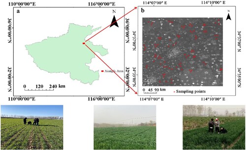
Figure 2. Flowchart of leaf area index inversion by GANNM.

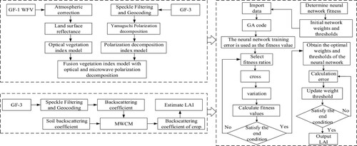
Table 1. Optical and microwave polarization decomposition vegetation index model.

Vegetation Index Type	Vegetation Index Name	Calculation Formula
Optical and microwave polarization decomposition vegetation index model	Modified normalized difference vegetation index	$\mathrm{M}\mathrm{N}\mathrm{D}\mathrm{V}\mathrm{I}=RV{I}_{Yamaguchi}\times \left[\left(P_{NIR}-P_R\right)/\left(P_{NIR}+P_R\right)\right]\times 10$	(3)
	Modified soil adjusted vegetation index	$\mathrm{M}\mathrm{S}\mathrm{A}\mathrm{V}\mathrm{I}=RV{I}_{Yamaguchi}\times \left[\left(P_{NIR}-P_R\right)\times \left(1+L\right)/\left(P_{NIR}-P_R+L\right)\right]$	(4)
	Modified ratio vegetation index	$\mathrm{M}\mathrm{R}\mathrm{V}\mathrm{I}=RV{I}_{Yamaguchi}\times \left[2.5\times P_{NIR}/P_R\right]$	(5)
	Modified enhanced vegetation index	$\mathrm{M}\mathrm{E}\mathrm{V}{\mathrm{I}}_2=RV{I}_{Yamaguchi}\times \left[2.5\times \left(P_{NIR}-P_R\right)/\left(P_{NIR}+2.4\times P_R+1\right)\right]\times 10$	(6)
	Modified soil adjusted vegetation index	$\mathrm{M}\mathrm{M}\mathrm{S}\mathrm{A}\mathrm{V}\mathrm{I}=RV{I}_{Yamaguchi}\times \left\{\left\{2\times P_{NIR}+1-\left[2\times P_{NIR}+1-{\left(2\times P_{NIR}+1\right)}^2-8\times {\left(P_{NIR}-P_R\right)}^{1/2}\right]\right\}/2\right\}$	(7)

Notes: $P_{NIR}$ and $P_R$ are the near infrared band, and red band of GF-1 WFV images, respectively. The reflectivity L is the soil-adjusted coefficient, and L = 0.5 in this paper.

Table 2. The range of all parameters in generating look up table

Name of parameter	Unit	Lower limit	Upper limit	Sources
$\mathrm{L}\mathrm{A}\mathrm{I}$	m^2/m^−2	0.1	7	Ground measurement
${\sigma }_{\mathrm{m}\mathrm{o}\mathrm{d}}$	dB	−12	−10	MWCM acquisition
${\sigma }_{\mathrm{o}\mathrm{b}\mathrm{s}}$	dB	−12	−10	Image acquisition
${\mathrm{M}}_{\mathrm{S}}$	%	5.9	40.1	Ground measurement
${\mathrm{f}}_{\mathrm{V}\mathrm{I}}$	No unit	0.15	0.45	Image acquisition

Table 3. Model accuracy index under different numbers of neurons in the hidden layer.

Equation	Number of Nodes in the Hidden Layer	R^2	RMSE
$H=\mathrm{l}\mathrm{o}{\mathrm{g}}_{2}I,I\in \left[0.002I,4I\right]$	9	0.419	0.675
	10	0.432	0.657
	11	0.536	0.569
	12	0.435	0.584
	13	0.389	0.663
$H=\sqrt{I+O}+\alpha ,\alpha \in \left[1,10\right]$	5	0.524	0.453
	6	0.513	0.456
	7	0.598	0.411
	8	0.532	0.492
	9	0.612	0.421
	10	0.787	0.253
	11	0.705	0.389
	12	0.695	0.401
	13	0.586	0.501
	14	0.553	0.536
$H=2I+1$	9	0.598	0.453
	10	0.602	0.436
	11	0.685	0.315
	12	0.632	0.376
	13	0.601	0.399

Table 4. Model accuracy index under different numbers of hidden layers.

Number of Hidden Layers	R^2	RMSE
1	0.645	0.501
2	0.686	0.423
3	0.753	0.256
4	0.769	0.235
5	0.721	0.386
6	0.683	0.429

Figure 3. The optical and microwave polarization decomposition vegetation index models. (a–e) are from the jointing, booting, heading, filling, and maturing stages, respectively.

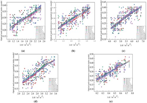
Table 5. Accuracy evaluation of the optical and microwave polarization decomposition vegetation index model.

Growth Stage	Model	R^2	RMSE	Growth Stage	Model	R^2	RMSE
Jointing	MEVI	0.632	0.3154	Booting	MEVI	0.584	0.3512
	MEVI2	0.624	0.3254		MEVI2	0.634	0.3189
	MSAVI	0.559	0.3910		MSAVI	0.623	0.3324
	MNDVI	0.723	0.2784		MNDVI	0.724	0.2746
	MMSAVI	0.589	0.3698		MMSAVI	0.574	0.3842
Heading	MEVI	0.631	0.3248	Filling	MEVI	0.624	0.3324
	MEVI2	0.658	0.2884		MEVI2	0.680	0.2995
	MSAVI	0.634	0.3125		MSAVI	0.664	0.2984
	MNDVI	0.684	0.2684		MNDVI	0.758	0.2839
	MMSAVI	0.569	0.3486		MMSAVI	0.612	0.3124
Maturing	MEVI	0.584	0.3784
	MEVI2	0.625	0.3012
	MSAVI	0.684	0.3284
	MNDVI	0.712	0.2735
	MMSAVI	0.634	0.3066

Figure 4. Correlation analysis between the backscattering coefficient model and LAI. (a–e) are from the jointing, booting, heading, filling, and maturing stages, respectively.

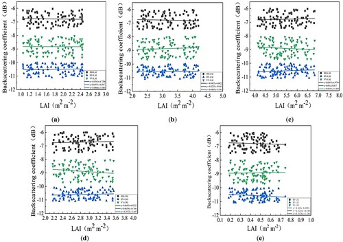
Table 6. Accuracy evaluation of the backscattering coefficient model.

Growth Stage	Model	R^2	RMSE	Growth Stage	Model	R^2	RMSE
Jointing	HH	0.165	0.9213	Booting	HH	0.151	0.9213
	HV	0.235	0.9010		HV	0.205	0.8922
	VV	0.155	0.9233		VV	0.113	0.9211
Heading	HH	0.159	0.9612	Filling	HH	0.166	0.9301
	HV	0.214	0.8966		HV	0.191	0.9011
	VV	0153	0.9362		VV	0.183	0.9266
Maturing	HH	0.112	0.9155
	HV	0.175	0.8863
	VV	0.153	0.9223

Figure 5. Correlation analysis of MWCM and LAI. (a–e) are from the jointing, booting, heading, filling, and maturing stages, respectively.

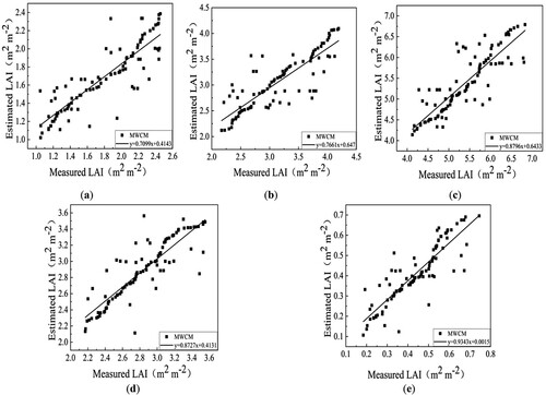
Table 7. Model parameters at HH, VV, and VH polarizations.

Polarization	Growth Stages	Model Parameters
		A	B	D	E
HV	Jointing	0.039	0.153	−11.20	19.52
	Booting	0.052	0.146	−12.12	15.33
	Heading	0.032	0.136	−9.21	16.24
	Filling	0.038	0.135	−10.32	13.25
	Maturing	0.042	0.201	−9.85	15.36

Table 8. MWCM accuracy evaluation.

Model	Growth Stages	R^2	RMSE
MWCM	Jointing	0.7622	0.4012
	Booting	0.7362	0.3988
	Heading	0.7476	0.4365
	Filling	0.7589	0.3842
	Maturing	0.7667	0.3822

Figure 6. Correlation analysis between BPNNM and GANNM models and LAI. (a–e) are from the jointing, booting, heading, filling, and maturing stages, respectively.

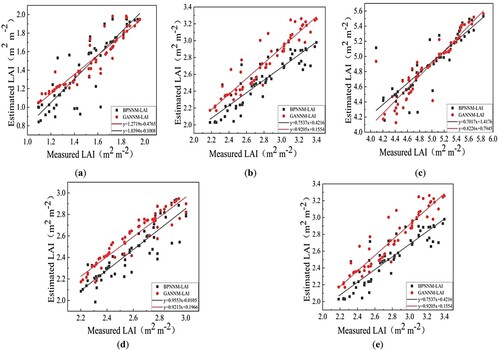
Table 9. Accuracy evaluation of the neural network model.

Model	Growth Stage	R^2	RMSE	Model	Growth Stage	R^2	RMSE
GANNM	Jointing	0.8223	0.2130	BPNNM	Jointing	0.7865	0.3021
	Booting	0.8924	0.1872		Booting	0.7897	0.2258
	Heading	0.9021	0.1675		Heading	0.7672	0.3245
	Filling	0.8121	0.1823		Filling	0.7897	0.2855
	Maturing	0.8536	0.1814		Maturing	0.7444	0.3542

Figure 7. The GANNM model and LAI verification analysis. (a–e) are from the jointing, booting, heading, filling, and maturing stages, respectively.

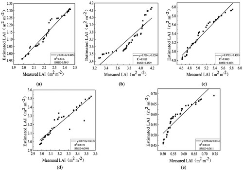
Figure 8. Correlation analysis between GF-3 LAI and MODIS LAI. (a–e) are from the jointing, booting, heading, filling, and maturing stages, respectively.

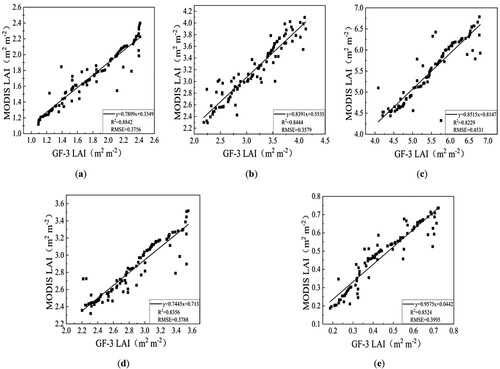
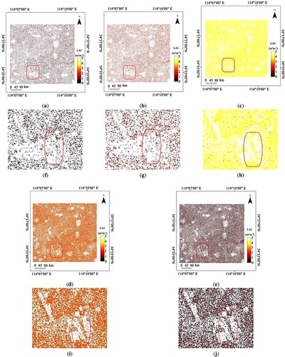
Figure 9. LAI images inverted by GANNM. (a–e) are from the jointing, booting, heading, filling, and maturing stages, respectively. (f–j) are the enlarged image from the (a–e) area.

Data availability statement

The code used in this study are available by contacting the corresponding author.