Underlying topography and forest height estimation from SAR tomography based on a nonparametric spectrum estimation method with low sidelobes

Figures & data

Figure 1. Geometry of an airborne TomoSAR imaging system over a forest area.

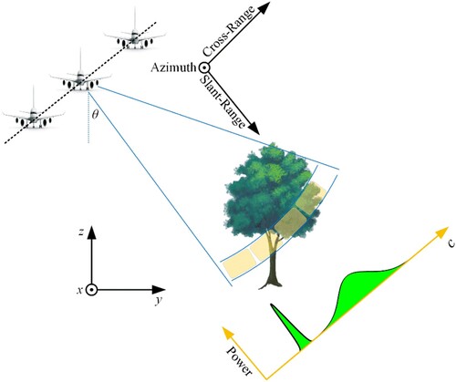
Table 1. The G-Pisarenko tomographic spectrum estimation method.

Initialization	$\mathit{R}={\displaystyle \frac{1}{L}\sum _{l=1}^L\mathit{U}\left(l\right)\mathit{U}(l{)}^{\mathrm{H}}}$
	$\left[\mathit{e},\mathit{\lambda }\right]=\mathrm{e}\mathrm{i}\mathrm{g}\left(\mathit{R}\right)$
	$\mu \mathrm{s}.\mathrm{t}.1={\displaystyle \frac{1}{L}\sum _{r=1}^N{\displaystyle \frac{{\lambda }_r}{{\lambda }_r-\mathit{\mu }}}}$
	$\hat{\mathit{R}}=0$
For n = 1: N
	$I_n=1+\left(1+\sum _{\begin{array}{c}k=1\\ k\ne n\end{array}}^N{\displaystyle \frac{{\lambda }_n}{{\lambda }_k-{\lambda }_n}-\sum _{k=1}^N{\displaystyle \frac{{\mu }_n}{{\lambda }_k-{\mu }_n}}}\right)\log {\lambda }_n+\sum _{\begin{array}{c}k=1\\ k\ne n\end{array}}^N{\displaystyle \frac{{\lambda }_k}{{\lambda }_k-{\lambda }_n}\log {\lambda }_k+\sum _{k=1}^N{\displaystyle \frac{{\mu }_k}{{\lambda }_n-{\mu }_k}\log {\mu }_k}}$
	$\hat{\mathit{R}}=\hat{\mathit{R}}+I_n{\mathit{e}}_n{\mathit{e}}_n^{\mathrm{H}}$
end
	${\hat{\mathit{P}}}_{\mathrm{G}\mathrm{P}}=\mathrm{e}\mathrm{x}\mathrm{p}\left({\mathit{A}}^{\mathrm{H}}\hat{\mathit{R}}\mathit{A}\right)$

Table 2. Parameters of the P-band F-SAR airborne SAR system.

Parameter	Value
Platform height	6096 m
Wavelength	0.6890 m
Incidence angle	20°−50°
Range resolution	3.84 m
Azimuth resolution	2 m
Polarization mode	HH + HV + VV

Table 3. Baseline information of the used datasets from the Lope region.

Identifier	Date of acquisition	Baseline (m)
FL06-PS02	10-Feb-2016	0
FL06-PS03		10
FL06-PS05		40
FL06-PS07		80
FL06-PS08		−20
FL06-PS11		−80

Figure 2. Comparison of the different methods for $\mathrm{\Delta }H=30\mathrm{m}$ with different SNRs: (a) SNR = 20 dB; (b) SNR = 5 dB.

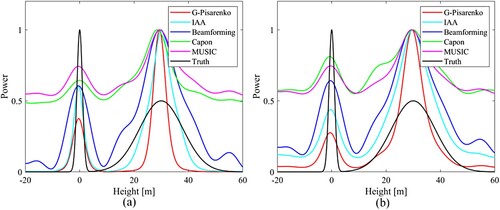
Figure 3. Comparison of the different methods for $\mathrm{\Delta }H=10\mathrm{m}$ with different SNRs: (a) SNR = 20 dB; (b) SNR = 5 dB.

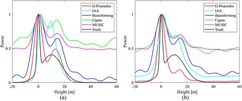
Figure 4. Comparison of different numbers of multi-looks ($L$) and images ($N$): (a) $L=100$, $N=6$; (b) $L=20$, $N=6$; (c) $L=100$, $N=4$.

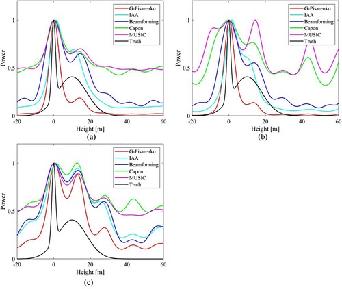
Figure 5. Normalized sidelobe levels for the SNR in different $\mathrm{\Delta }H$ values: (a) $\mathrm{\Delta }H=10$ m; (b) $\mathrm{\Delta }H=30$ m.

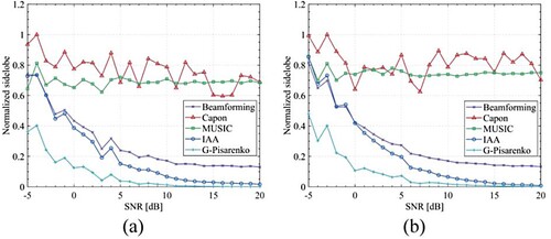
Figure 6. (a) Gabon, Africa (green polygon) and (b) the Pauli RGB image of the study area.

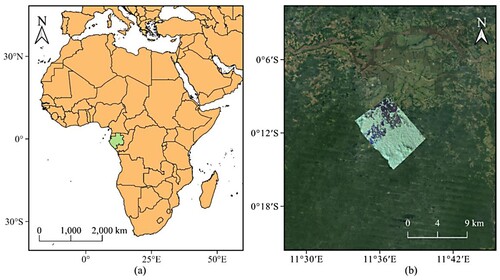
Figure 7. The distribution of the forest backscattering mechanism power with elevation.

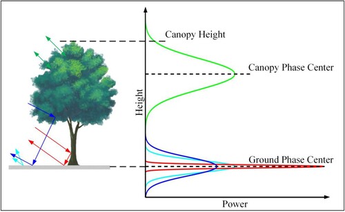
Figure 8. Selected profile (red solid line) on the Pauli RGB image.

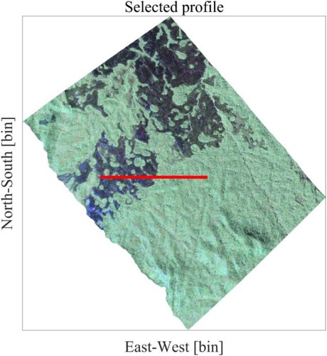
Figure 9. Tomograms of the HH (left column), HV (middle column), and VV (right column) channels on the selected range profile: (a), (f), and (k) Beamforming; (b), (g), and (l) Capon; (c), (h), and (m) MUSIC; (d), (i), and (n) IAA; (e), (j), and (o) G-Pisarenko. The black solid lines and white dotted lines denote the LiDAR DTM and CHM, respectively.

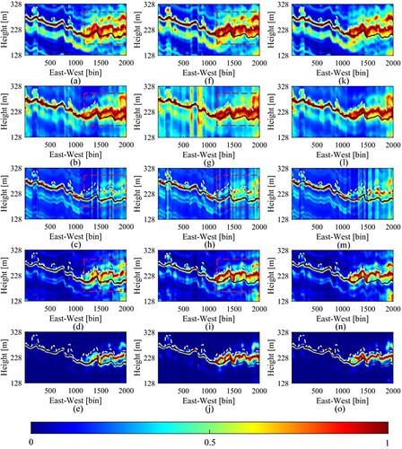
Figure 10. The estimated results obtained by the TomoSAR methods for the selected profile: (a) underlying topography, (b) forest canopy.

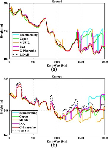
Table 4. Running times of the different methods for estimating the selected profile.

Method	Time [s]
Beamforming	70
Capon	84
MUSIC	69
IAA	87
G-Pisarenko	238

Figure 11. Estimated DTMs: (a) Beamforming, (b) Capon, (c) MUSIC, (d) IAA, (e) G-Pisarenko; referenced DTM: (f) LiDAR.

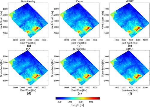
Figure 12. 2D joint distribution between the LiDAR DTM measurements and the estimations of the five methods for the selected range profile: (a) Beamforming, (b) Capon, (c) MUSIC, (d) IAA, (e) G-Pisarenko.

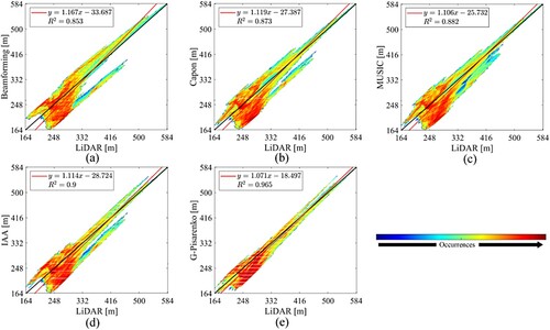
Table 5. The mean error and RMSE of the different methods for the underlying topography of the whole study area.

Method	Mean error (m)	RMSE (m)
Beamforming	4.95	9.15
Capon	4.49	8.72
MUSIC	3.96	8.28
IAA	3.67	8.03
G-Pisarenko	2.81	7.26

Figure 13. RMSE between the LiDAR CHM and TomoSAR CHM with different power loss values.

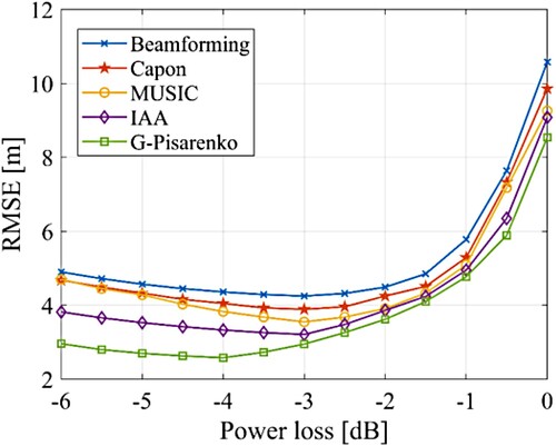
Figure 14. Estimated CHM: (a) Beamforming, (b) Capon, (c) MUSIC, (d) IAA, (e) G-Pisarenko; referenced CHM: (f) LiDAR.

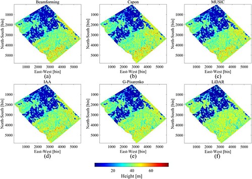
Table 6. The mean error and RMSE of the different methods for the forest heights of the whole study area.

Method	Mean error (m)	RMSE (m)
Beamforming	−0.38	4.25
Capon	−0.35	3.89
MUSIC	−0.18	3.55
IAA	−0.25	3.21
G-Pisarenko	−0.23	2.58

Figure 15. 2D joint distribution between the LiDAR CHM measurements and the estimations of the five methods for the selected range profile: (a) Beamforming, (b) Capon, (c) MUSIC, (d) IAA, (e) G-Pisarenko.

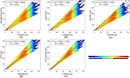
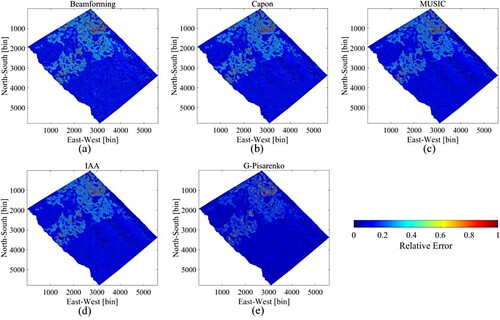
Figure 16. The estimated CHM relative error: (a) Beamforming w.r.t LiDAR, (b) Capon w.r.t LiDAR, (c) MUSIC w.r.t LiDAR, (d) IAA w.r.t LiDAR, (e) G-Pisarenko w.r.t LiDAR.