A hybrid model for high spatial and temporal resolution population distribution prediction

Figures & data

Table 1. Comparison of conventional, model-based ML, and the proposed hybrid methods

Category	Method	Temporal scale	Spatial scale	Object	Pros	Cons
Conventional	Linear regression	Year	Region	Population	Good interpretability	Poor accuracy
	ARIMA	Year	Country	Population	Better accuracy	Low efficiency for handling big data
Model-based	CGM	Hour	10 km*10 km for a city	GPS trace	Good interpretability	Requiring much more prior knowledge, low temporal, and spatial granularity
	CA	Second	A house	Evacuation	High suitability for natural processes
Machine learning	CNN	Year	1 km × 1 km for a country	people flow	High suitability for image data,	Less interpretability, high accuracy when combined with model-based method
	LSTM	Hour	1 km × 1 km for a city	Crowd flow	time series data and
	Tree	5 min	600 m × 600 m for a city	People movement	classification problems
Hybrid	CA + ANN	Year	1 km × 1 km for a region	Land expansion	Excellent accuracy and interpretability	No consideration of temporal information
	CA + LSTM	Less than one year	Smaller than 1 km × 1 km for a region	Earth system	Consideration of spatial and temporal information	Challenge in transferability

Figure 1. Framework of this study.

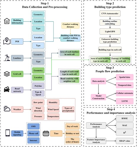
Figure 2. Road network of Milan.

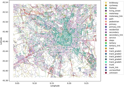
Table 2. Details of collected data

Name	Explanation	Type
POI	Position, type of each POI	Point
Building	Position, shape and type of each building	Geometry
Road	Position, shape and type of each road	Line
Land use	Position, shape and type of land use	Geometry
Weather	Seven weather factors for each hour	String/Continuous
Mobile phone signalling	The number of mobile signalling in each cell and each hour	Integer
Grid cell	Position and shape of each 235m × 235 m cell	Geometry

Figure 3. Distribution of land use in Milan.

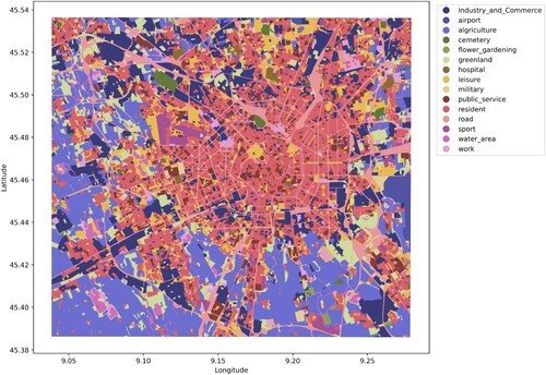
Figure 4. Distribution of one week of mobile phone usage in Milan as a high-resolution grid cell.

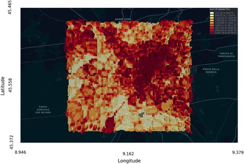
Figure 5. Data pre-processing workflow.

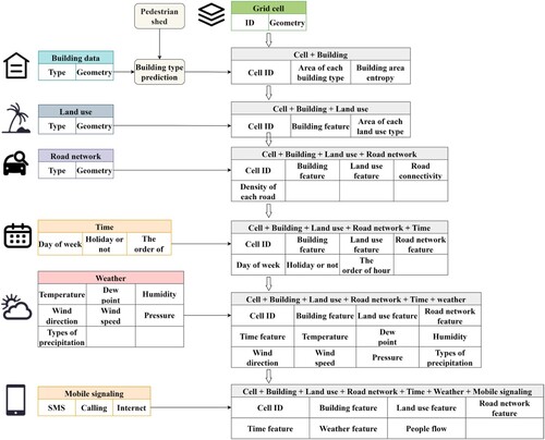
Figure 6. Process of predicting building type.

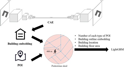
Figure 7. Example of (a) Moore and (b) diamond-shaped neighbourhood.

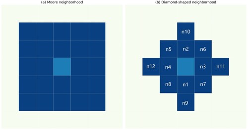
Figure 8. Process of combing CA and LSTM.

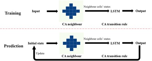
Figure 9. Structure of CAE.

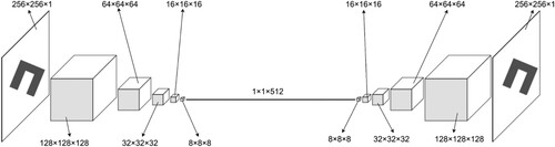
Figure 10. Examples of (a) building outlines and (b) their reconstruction.

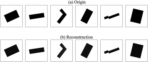
Figure 11. All building distribution in Milan after prediction.

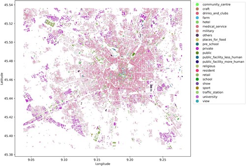
Table 3. Setting and result of LightGBM.

Name of parameters	The range of parameters	Optimal parameter
Number of leaves	20, 50, 100, 200, 350, 500, 800, 1000	500
Max depth	5, 10, 20, 40, 60, 80, 100	40
Learning rate	0.002, 0.004, 0.006, 0.008,0.1	0.004

The ratio of the training and testing sets was 7:3, the F1-score was 0.902, and the accuracy was 86.8%. Figure 11 shows the prediction outcome of building distribution in Milan.

Figure 12. Relationship between temperature, building density, and population distribution.

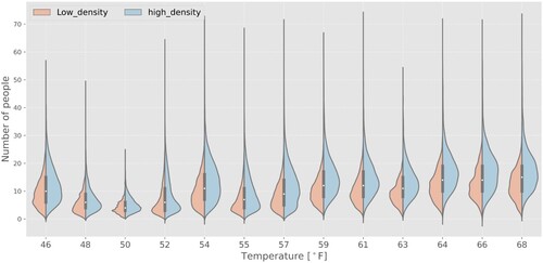
Figure 13. Population distribution of various land use (a–o) and grid cells (p).

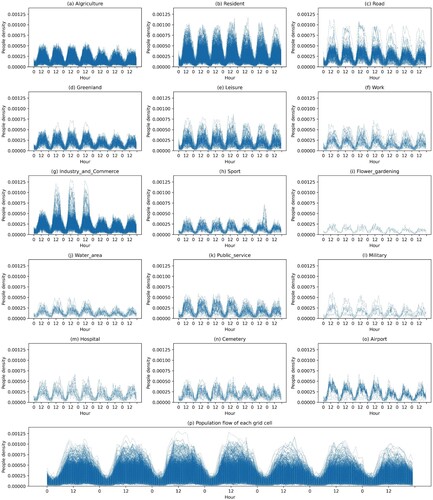
Figure 14. Relationship between dew point (a), humidity (b), wind speed (c), pressure (d), temperature, wind direction (e), and population distribution; the black line is the median value, and the white line is the mean value.

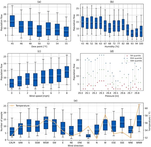
Figure 15. Cosine similarity between grid cells on days of a week for land use types.

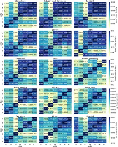
Figure 16. Autocorrelation of population distribution for grid cells in different land use types.

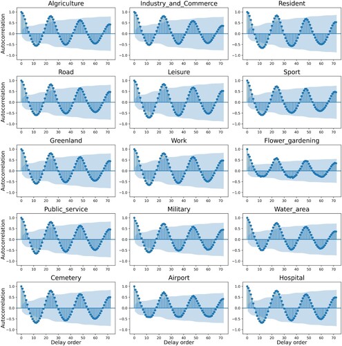
Figure 17. Training process of proposed model.

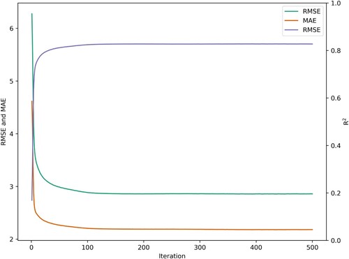
Figure 18. Comparison of proposed model and other three models (baseline, CA + BPNN, and LSTM)

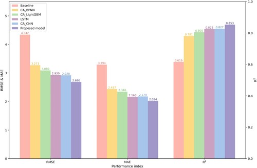
Figure 19. Importance of each variable (n1 to n12 refers to the code of neighbour cells shown in Figure 7).

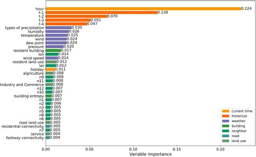
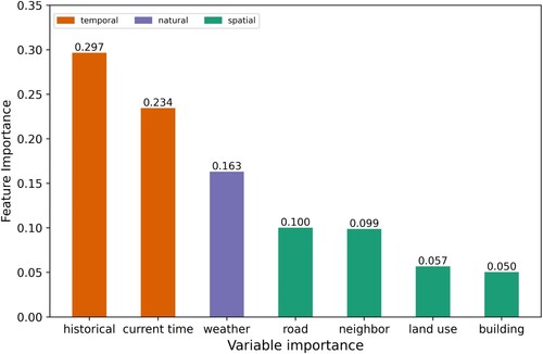
Figure 20. Importance of each category.

Data availability statement

The authors confirm that the data supporting the findings of this study are available within the article.