Figures & data
Figure 1. Technical routine.
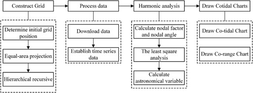
Figure 2. Vertex and cells coding on an unfolded icosahedron.
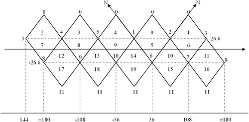
Figure 3. Spherical hexagonal discrete global based on an icosahedron.
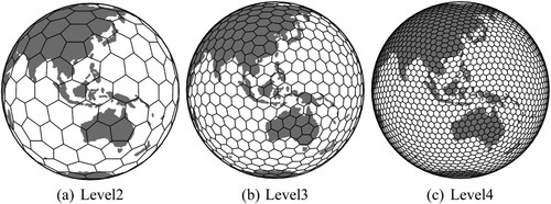
Table 1. Resolution of the global equal-area hexagonal grid.
Table 2. Satellite data storage structure after processing.
Figure 4. Satellite altimeter sequence data of several points.
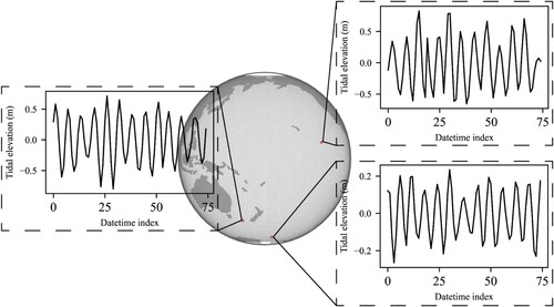
Figure 5. Schematic diagram of tidal elevation sequence of compound tide and major constituent tides derived from harmonic constants.
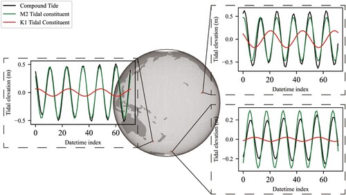
Figure 6. Flow chart of calculating harmonic constants.
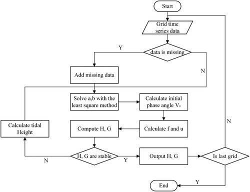
Figure 7. Schematic diagram of diffusing query adjacent neighbour: (a) first layer diffusion; (b) second layer diffusion; (c) third layer diffusion.
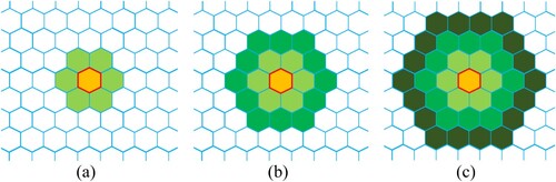
Figure 8. Steps for searching equivalent grids: (a) grid classification; (b) category boundary; (c) query higher level grid boundary; (d) the equivalent grids under higher level grid.
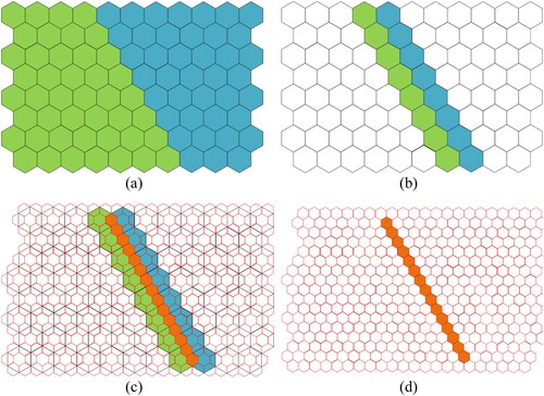
Figure 9. An example diagram of Cotidal Chart.
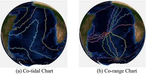
Figure 10. Jason series satellite ground tracks of global ocean.
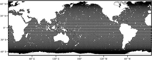
Table 3. Introduction of altimeter data.
Figure 11. Location distribution of gauge stations.
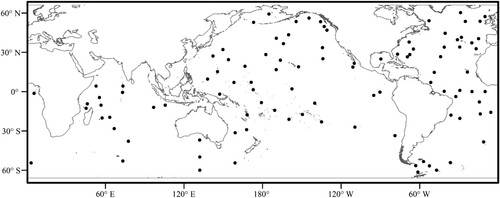
Figure 12. Comparison of the TPXO9.5 ocean model and simulated results for the tidal constituent M2.
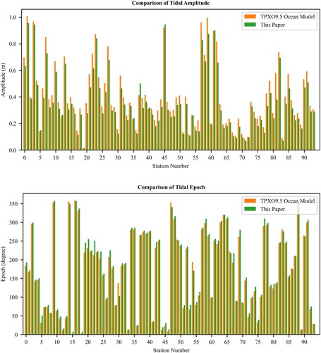
Table 4. RMSE values of eight components at gauge stations.
Figure 13. Comparison of the RMSE for the simulation results obtained using the two grids.
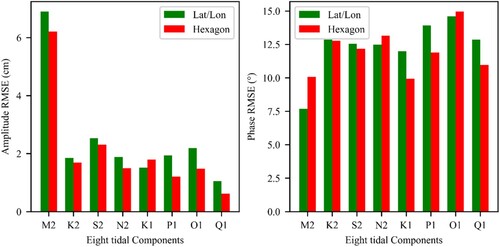
Figure 14. Co-tidal Charts and Co-range Charts of M2 components in three oceans. Left are Co-tidal charts and right are Co-range charts.
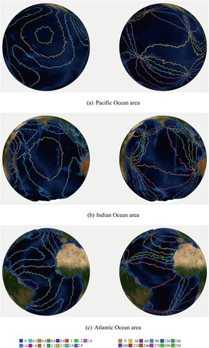
Figure 15. Tidal elevation was retrieved from eight major constituents: (a) Global Ocean tidal elevation; (b) Indian Ocean tidal elevation; (c) Pacific Ocean tidal elevation; (d) Atlantic Ocean tidal elevation.
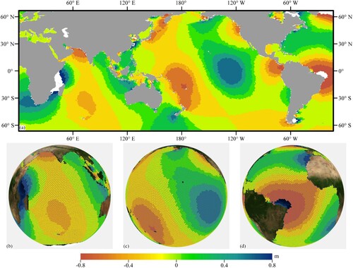
Figure 16. Comparison of RMSE of two types of grid in different latitude intervals.
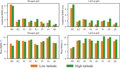
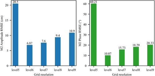
Figure 17. RMSE-Amplitude (left), RMSE-Phase (right).