Figures & data
Figure 1. (a) The spatial distribution of the POI data and the road data. (b) Overview of the study area. (c) The spatial distribution of the POI kernel density. (d) The spatial distribution of three levels of the road network.
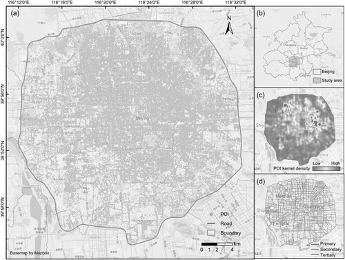
Figure 2. Rank-frequency plot for POI Sub-types. (a) Rank-frequency plot and (b) Rank-frequency log plot.
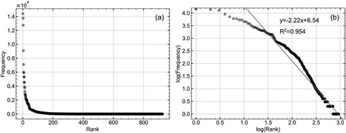
Figure 3. An overall framework of the proposed approach.
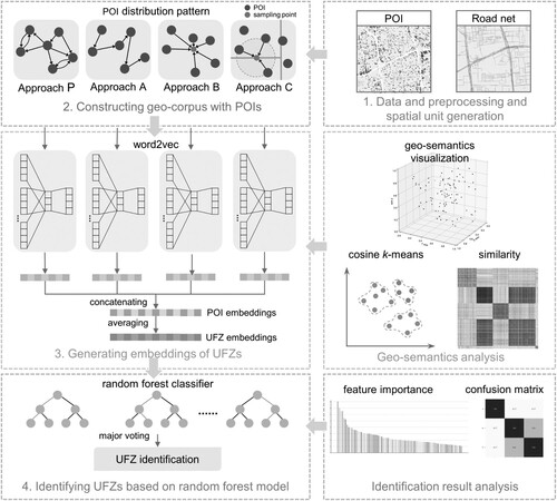
Figure 4. POI taxonomy tree map for 12 Big-types with 100 Mid-types.
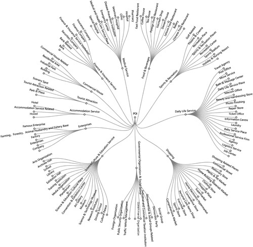
Figure 5. Obtaining spatial units based on road network.
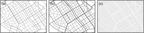
Figure 6. The process of the proposed geo-corpus construction approach.
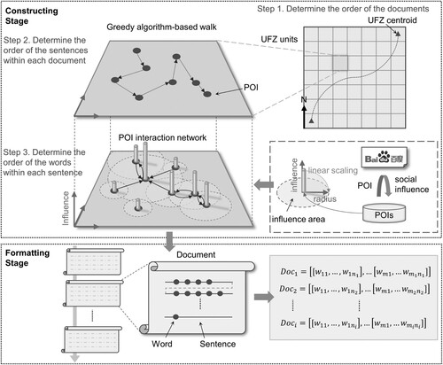
Figure 7. Schematic diagram of the geo-corpus construction approaches. (a) Approach A. (b) Approach B. (c) Approach C.
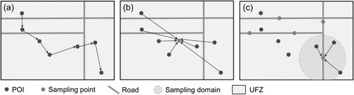
Table 1. Experiments design based on four combination modes.
Figure 8. POI-type semantic subspace with a local space.
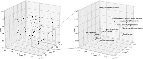
Figure 9. The pairwise similarities between UFZs.
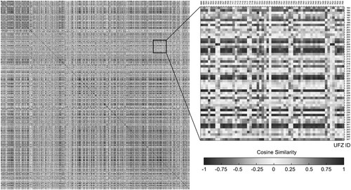
Figure 10. Changes of clustering effect of different K values.
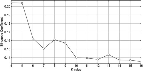
Figure 11. The pairwise similarity between UFZs ranked by K-means-based cluster, and locations and remote sensing images of the six sample zones in cluster #4.
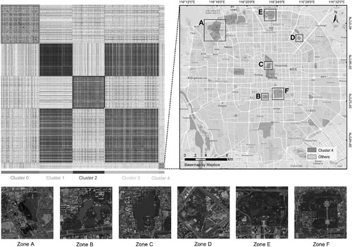
Figure 12. The matrix of OOB accuracy with different combinations of max_features and n_estimators.
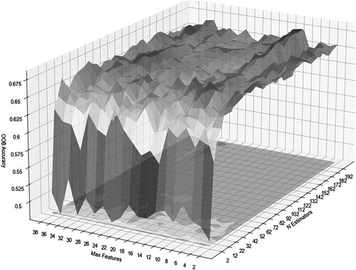
Figure 14. Classification results of UFZs. (0) Ground truth. (1) ∼ (15) Results of experiment 1 ∼ 15, and experiment 15 corresponds to our proposed method. Sparse zones refer to spatial units that are excluded from the study.
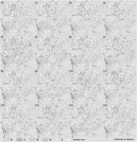
Table 2. Confusion matrix of classification results. (R: residential zone. A: administrative and public service zone. M: industrial zone. B: business zone. G: green space).
Figure 13. Feature variable importance ranking for UFZ classification.
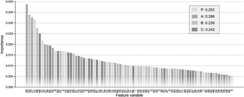
Table 3. Accuracy evaluation. (*: feature combination mode. R: residential zone. A: administrative and public service zone. M: industrial zone. B: business zone. G: green space).
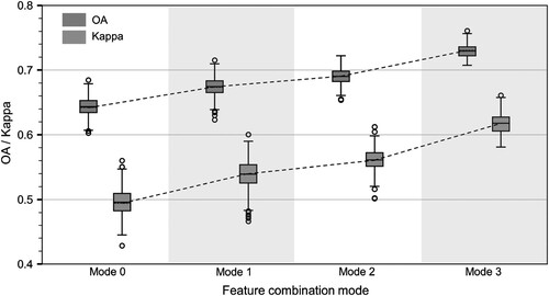
Figure 15. Box plot of different feature combination modes.