Adaptive step-size forward advection method for aerosol process simulation

Figures & data

Figure 1. Methods framework diagram.

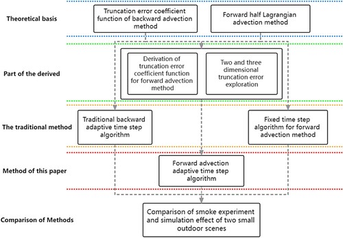
Figure 2. Schematic diagram of the traditional semi-Lagrangian advection method.

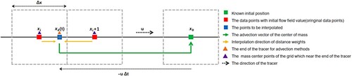
Figure 3. Schematic diagram of the forward semi-Lagrangian advection method.

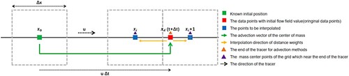
Figure 4. Schematic representation of 3D first-order forward advection interpolation.

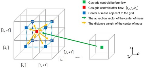
Figure 5. Mass collection process of grid centroid points in forward advection method.

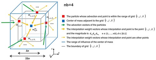
Figure 6. Comparison test of mass conservation between traditional semi-Lagrangian method and forward method under closed condition.

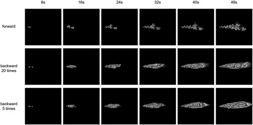
Figure 7. Quality errors of the traditional semi-Lagrangian and forward methods under closed conditions.

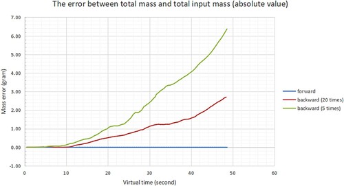
Table 1. Comparison of input quality and output quality of the forward method under closed condition.

t	m1 (mass of input)	m2 (mass of output)	m1-m2
4.5	0.200893	0.200893	−1.49E-08
5.02232	0.222128	0.222128	−4.47E-08
5.5532	0.244161	0.244161	−2.98E-08
6.10403	0.267116	0.267116	5.96E-08
…	…	…	…
47.1115	1.90457	1.90449	7.89E-05
47.6142	1.92467	1.92459	7.53E-05
48.1167	1.94476	1.94469	6.94E-05
48.6189	1.96484	1.96476	7.82E-05

Figure 8. Schematic diagram of first-order backward and forward interpolation. Red points are original value points, and blue points are to be interpolated. $x_i$ and $x_{i+1}$ are the centre points of the neighbourhood grid. (a) Backward interpolation. (b) Forward interpolation.

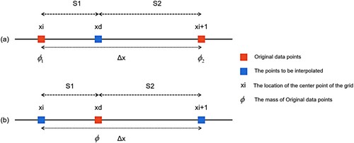
Figure 9. First-order one-dimensional backward tracking truncation error coefficient function image.

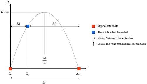
Figure 10. Schematic diagram of forward interpolation mirror deformation method.

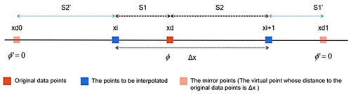
Figure 11. First-order one-dimensional forward advection truncation error coefficient function.

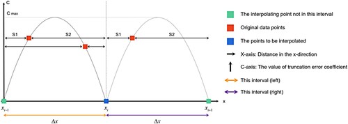
Figure 12. Forward method two-advection endpoint distribution types.

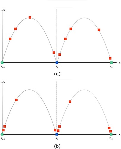
Figure 13. Interpolation characteristics of different CFL values of X-axis components.

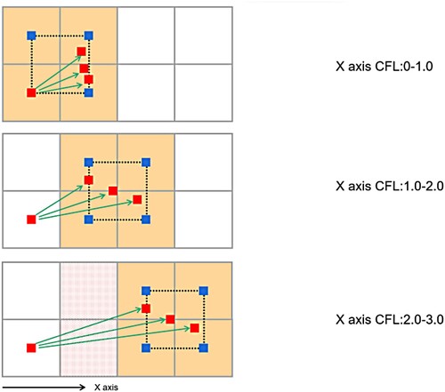
Figure 14. Slope setting of flow direction.

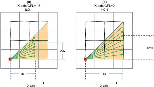
Figure 15. Schematic diagram of slope in 3D.

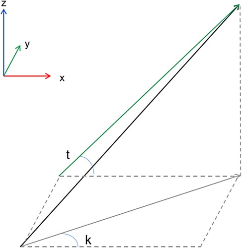
Figure 16. Truncation error coefficient functions of different slope components.

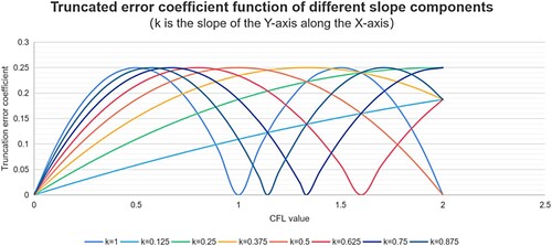
Figure 17. Two-dimensional truncation error coefficient function image.

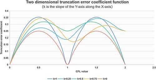
Figure 18. Four three-dimensional truncation error coefficient function images of t-slope.

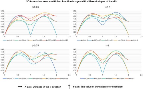
Figure 19. Tilted photographic model of the experimental area.

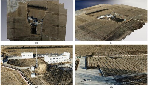
Table 2. Evaluation criteria of Kappa index.

Kappa value	Evaluate
0.0–0.20	Extremely low consistency
0.21–0.40	General consistency
0.41–0.60	Medium consistency
0.61–0.80	High degree of consistency
0.81–1.0	Almost identical

Figure 20. Comparison between full-scale simple terrain experiment and simulation results.

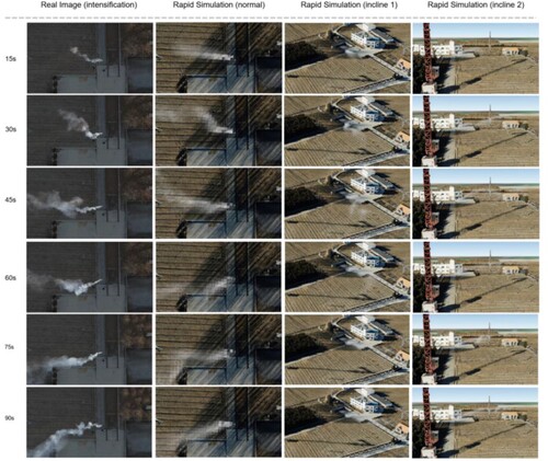
Figure 21. Comparison of full-scale complex terrain experiment and simulation results.

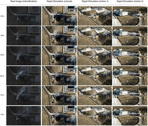
Figure 22. Adaptive time step change image. (a) simple terrain experiment; (b) complex terrain experiment.

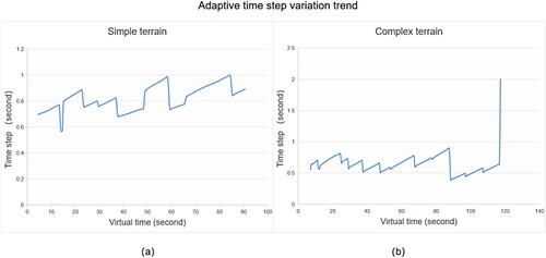
Figure 23. Comparison of intersection between simple terrain forward adaptive step size and fixed time step size methods.

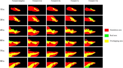
Figure 24. Comparison of the intersection of forward adaptive step size and fixed time step size methods for complex terrain.

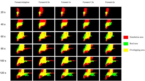
Table 3. Average Kappa values of forward adaptive step size and fixed time step size in simple and complex terrain experiments.

Terrain	Different time step groups
	Forward adaptive	0.2 s	0.5 s	1 s	1.5 s	2 s
Simple terrain	0.47154	0.34269	0.39306	0.46582	0.44044
Complex terrain	0.63513		0.60287	0.61411	0.58263	0.58148

Figure 25. Comparison of the intersection of forward and backward adaptive step sizes in simple terrain experiment.

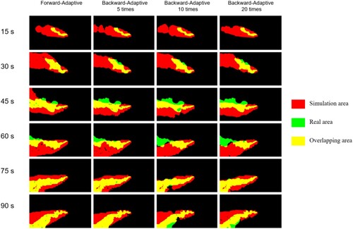
Figure 27. Time trend calculation of forward and backward adaptive steps for two terrain experiments.

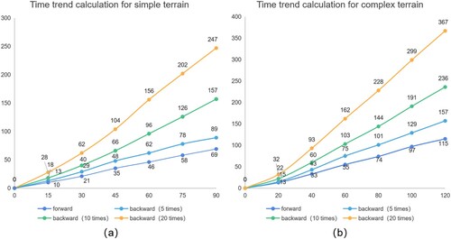
Table 4. Average Kappa values of forward and backward adaptive step sizes in two terrain experiments.

Terrain	Different advection calculation methods
	Forward adaptive	Backward (5 times)	Backward (10 times)	Backward (20 times)
Simple terrain	0.47154	0.46792	0.44044	0.42665
Complex terrain	0.63513	0.62043	0.15709	0.30997

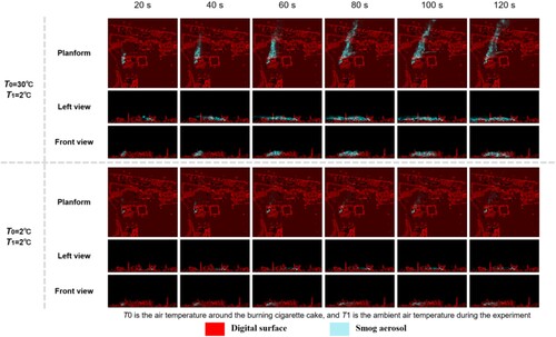
Figure 28. Three-dimensional motion visualisation of smoke aerosol in simple terrain under two temperature differences.

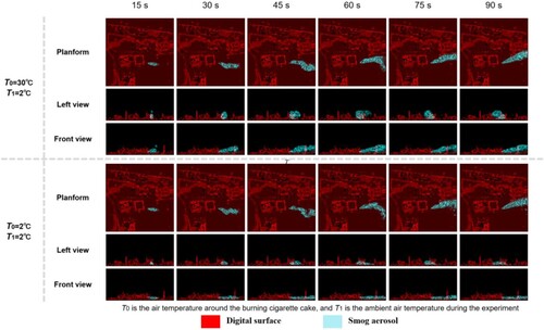
Figure 26. Comparison of the intersection of forward and backward adaptive step sizes in complex terrain experiment.

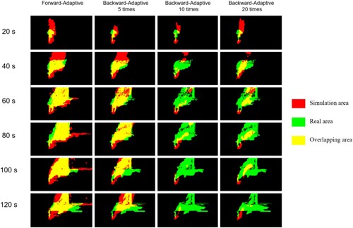
Figure 29. Three-dimensional motion visualisation of smoke aerosol in complex terrain under two temperature differences.