Machine learning-based prediction of sand and dust storm sources in arid Central Asia

Figures & data

Figure 1. Geographical location of the study area and spatial distribution of the main deserts in ACA.

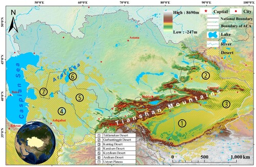
Figure 2. Flowchart of this study in the GEE platform. See Table 1 for detailed land/climate variables.

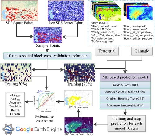
Figure 3. Thematic maps of SDS source effective predictor variables and RGB image. (a) DLSTR. (b) Vol_Wt_S. (c) LCT. (d) Wt_C. (e) NDVI. (f) So_Sa. (g) Slope. (h) So_Wt. (i) Sur_R. (j) Wd_Sp. (k) Sn_C. (l) A_Temp. (m) T_Prec. (n) So_Temp. (o) RGB image.

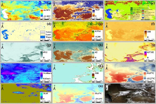
Table 1. Summary of the input variables in this study.

Category	Variable	Spatial Resolution	Temporal Resolution	Temporal Coverage	Source/Reference
Terrestrial factors	DLSTR	1000 m	daily	2003–2020	AGCD (Li et al. 2018)
	Vol_Wt_S	11132 m	hourly	1982 to present	ERA5 (Hersbach et al. 2018)
	LCT	500 m	yearly	2001 to present	MCD12Q1 (Friedl and Sulla-Menashe 2019)
	Wt_C	30 m	yearly	1984–2021	JRC_GSW (Pekel et al. 2016)
	NDVI	250 m	16-Day	2000 to present	MOD13Q1 (Didan 2021)
	So_Sa	250 m	-	-	OpenLandMap (Hengl 2018)
	Slope	90 m	-	-	SRTM_DEM (Jarvis et al. 2008)
	So_Wt	250 m	-	-	OpenLandMap (Hengl and Gupta 2019)
	Sur_R	90 m	-	-	Geomorpho90 m (Amatulli et al. 2020)
Climatic factors	Wd_Sp	11132 m	hourly	1982 to present	ERA5 (Hersbach et al. 2018)
	Sn_C	11132 m	hourly	1982 to present	ERA5 (Hersbach et al. 2018)
	A_Temp	11132 m	hourly	1982 to present	ERA5 (Hersbach et al. 2018)
	T_Prec	11132 m	hourly	1982 to present	ERA5 (Hersbach et al. 2018)
	So_Temp	11132 m	hourly	1982 to present	ERA5 (Hersbach et al. 2018)

Table 2. Performance evaluation of four ML based models.

ML Models	TA	VA	Precision	Recall	F1 Score	AUCROC	AUCPR
RF	0.998	0.875	0.811	0.889	0.847	0.949	0.918
SVM	0.886	0.860	0.793	0.862	0.824	0.920	0.877
GBT	0.994	0.856	0.793	0.866	0.827	0.931	0.887
MaxEnt	0.872	0.859	0.772	0.888	0.825	0.934	0.897

Figure 4. ROC curves for the four methods in SDS source susceptibility prediction based on nine model iterations.

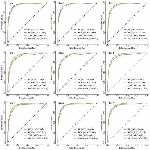
Figure 5. PR curves for the four methods in SDS source susceptibility prediction based on nine model iterations.

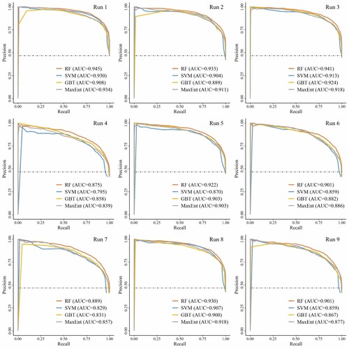
Figure 6. SDS source susceptibility maps produced via the ML-based methods in spring. (a) 2008-4-29, (b) 2016-5-11, (c) 2018-4-18.

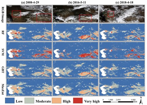
Figure 7. SDS source susceptibility maps produced using the ML-based methods in summer and autumn. (d) 2010-8-26, (e) 2015-6-10, (f) 2019-9-24.

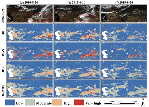
Figure 8. SDS source susceptibility maps produced using the ML-based methods in winter. (g) 2007-3-1, (h) 2013-1-23, (i) 2019-1-2.

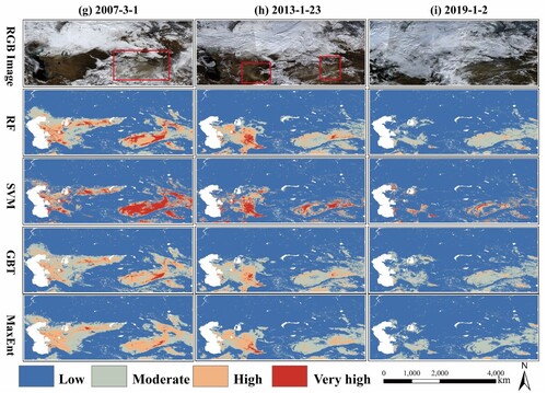
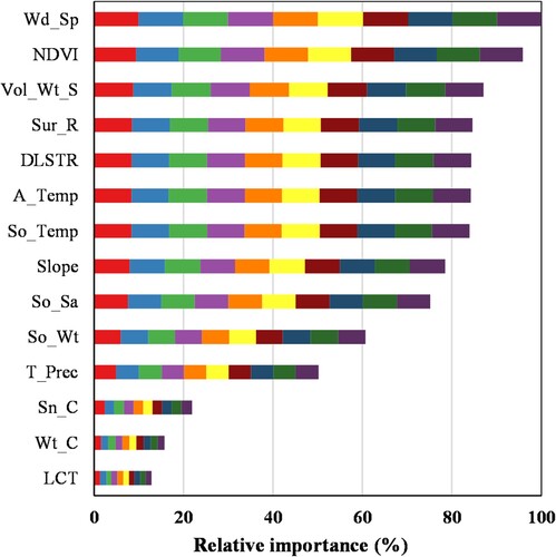
Figure 9. Relative importance of the variables to the prediction model outputs based on the random forest.

Li, Xiaoma, Yuyu Zhou, Ghassem R. Asrar, and Zhengyuan Zhu. 2018. “Creating a Seamless 1 km Resolution Daily Land Surface Temperature Dataset for Urban and Surrounding Areas in the Conterminous United States.” Remote Sensing of Environment 206: 84–97. doi: 10.1016/j.rse.2017.12.010.

 Web of Science ®Google Scholar

Hersbach, H., B. Bell, P. Berrisford, G. Biavati, A. Horányi, J. Muñoz Sabater, J. Nicolas, C. Peubey, R. Radu, and I. Rozum. 2018. “ERA5 hourly data on single levels from 1979 to present.” In, edited by Copernicus Climate Change Service (C3S) Climate Data Store (CDS).

 Google Scholar

Friedl, M., and D. Sulla-Menashe. 2019. “MCD12Q1 MODIS/Terra+Aqua Land Cover Type Yearly L3 Global 500 m SIN Grid V006.” In.: NASA EOSDIS Land Processes DAAC.

 Google Scholar

Pekel, Jean-François, Andrew Cottam, Noel Gorelick, and Alan S. Belward. 2016. “High-Resolution Mapping of Global Surface Water and Its Long-Term Changes.” Nature 540 (7633): 418–422. doi: 10.1038/nature20584.

 PubMed Web of Science ®Google Scholar

Didan, K. 2021. “MODIS/Terra Vegetation Indices 16-Day L3 Global 250 m SIN Grid V061.” In.: NASA EOSDIS Land Processes DAAC.

 Google Scholar

Hengl, Tomislav. 2018. “Sand content in % (kg / kg) at 6 standard depths (0, 10, 30, 60, 100 and 200 cm) at 250 m resolution (Version v02).” In.: Zenodo.

 Google Scholar

Jarvis, Andy, Hannes Isaak Reuter, Andrew Nelson, and Edward Guevara. 2008. “Hole-filled SRTM for the globe Version 4.” In.: CGIAR-CSI SRTM 90 m Database.

 Google Scholar

Hengl, Tomislav, and Surya Gupta. 2019. “Soil Water Content (volumetric %) for 33kPa and 1500kPa Suctions Predicted at 6 Standard Depths (0, 10, 30, 60, 100 and 200 cm) at 250 m resolution (Version v01).” In.: Zenodo.

 Google Scholar

Amatulli, Giuseppe, Daniel McInerney, Tushar Sethi, Peter Strobl, and Sami Domisch. 2020. “Geomorpho90m, Empirical Evaluation and Accuracy Assessment of Global High-Resolution Geomorphometric Layers.” Scientific Data 7 (1): 162. doi: 10.1038/s41597-020-0479-6.

 PubMed Web of Science ®Google Scholar