Spectral clustering eigenvector selection of hyperspectral image based on the coincidence degree of data distribution

Figures & data

Figure 1. Study area and hyperspectral data. (a) location map; (b) mineral distribution map; (c) AVIRIS image.

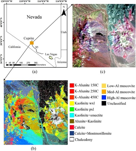
Figure 2. Flowchart of the clustering-matching mapping procedure of spectral clustering based on various eigenvector selection methods.

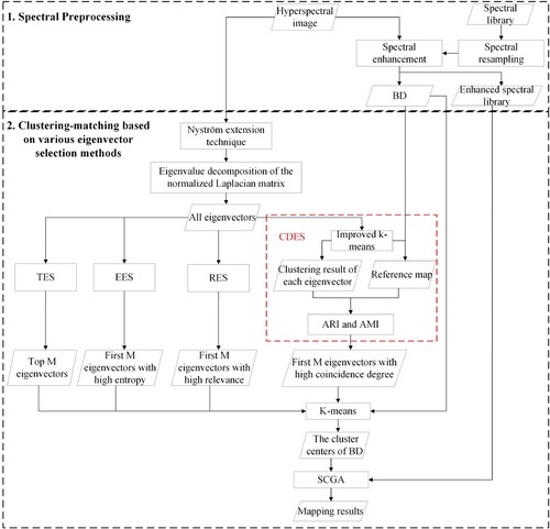
Figure 3. Clustering results of conventional k-means (a) and improved k-means (b).

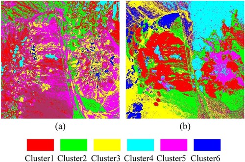
Table 1. Contingency table.

U/G	$G_1$	$G_2$	$\cdots$	$G_C$	Sums
$U_1$	$n_{11}$	$n_{12}$	$\cdots$	$n_{1C}$	$a_1$
$U_2$	$n_{21}$	$n_{22}$	$\cdots$	$n_{2C}$	$a_2$
$⋮$	$⋮$	$⋮$	$\ddots$	$⋮$	$⋮$
$U_R$	$n_{R1}$	$n_{R2}$	$\cdots$	$n_{RC}$	$a_R$
Sums	$b_1$	$b_2$	$\cdots$	$b_c$	$\sum _{ij}{n}_{ij}=N$

Figure 4. ARI (a) and AMI (b) values of unsorted original eigenvectors based on the mineral distribution map and reference map.

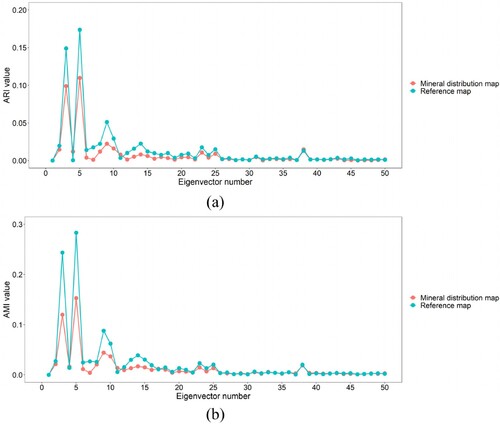
Figure 5. Flowchart of CDES

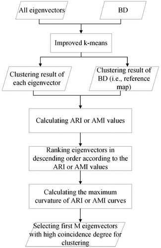
Figure 6. Scatter diagram for determining the $M$ value. The red dot represents the point with the maximum curvature.

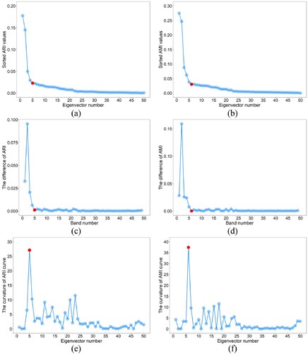
Figure 7. Bar diagram for selecting the eigenvectors stably. Here, (a) and (b) are the eigenvector selection results of ARI and AMI based on 100 random k-means clustering, respectively, and the percentage in the bar graph represents the maximum probability that an eigenvector is selected at each ranking position. (c) and (d) are the $M$ values determined by calculating the maximum curvature of the ARI and AMI curves, respectively.

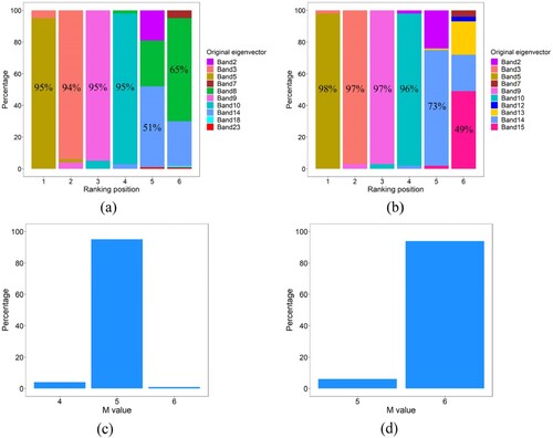
Figure 8. First six eigenvectors selected by various eigenvector selection methods.

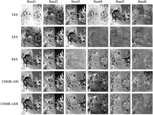
Figure 9. Boxplots for analysing the stability of the six CDES methods in eigenvector selection. (a), (b), (c), (d), (e), and (f) are the first to the sixth selected eigenvectors, respectively.

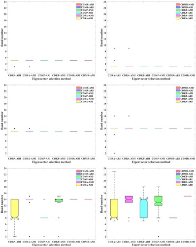
Figure 10. Mineral mapping results of spectral clustering. (a1–a6), (b1–b6), (c1–c6), (d1–d6), and (e1–e6) are the mineral mapping results of TES, EES, RES, CDMR-ARI, and CDMR-AMI respectively. The mapping results of columns 1 to 6 are based on the first to the first six eigenvectors respectively.

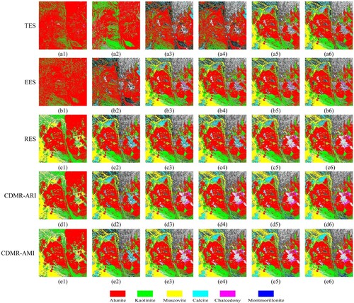
Table 2. Mineral mapping accuracies of various eigenvector selection methods.

	OA						KC
	1	2	3	4	5	6	1	2	3	4	5	6
TES	0.42	0.40	0.41	0.41	0.73	0.73	0.14	0.20	0.24	0.25	0.66	0.66
EES	0.38	0.41	0.72	0.72	0.72	0.72	0.09	0.25	0.65	0.65	0.66	0.65
RES	0.62	0.75	0.77	0.77	0.78	0.79	0.52	0.68	0.70	0.70	0.72	0.74
CDRA-ARI	0.61	0.74	0.81	0.85	0.81	0.82	0.51	0.68	0.76	0.80	0.76	0.77
CDRA-AMI	0.61	0.74	0.81	0.84	0.83	0.81	0.52	0.68	0.76	0.80	0.79	0.76
CDKP-ARI	0.62	0.75	0.82	0.85	0.80	0.83	0.52	0.68	0.77	0.81	0.75	0.78
CDKP-AMI	0.62	0.75	0.82	0.85	0.84	0.80	0.52	0.68	0.77	0.81	0.79	0.75
CDMR-ARI	0.62	0.75	0.82	0.85	0.86	0.84	0.52	0.68	0.77	0.81	0.82	0.80
CDMR-AMI	0.62	0.75	0.82	0.85	0.86	0.85	0.52	0.68	0.77	0.81	0.82	0.81

Figure 11. Mapping accuracies of TES (a), EES (b), RES (c), CDMR-ARI (d), and CDMR-AMI (e) with different eigenvectors. In particular, the coral line in figure (c) represents the relevance values of each eigenvector, and the threshold of 0.5 corresponds to the first seventeen eigenvectors. The red dot represents the point with the maximum mapping accuracy.

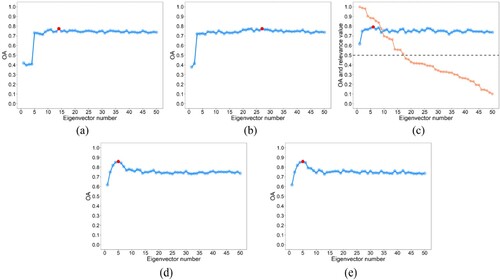
Table 3. Running time of various eigenvector selection methods.

Selection Method	Time(min)	Selection Method		Time(min)
TES	0.00	CDRA	ARI	0.17
			AMI	0.17
EES	607.19	CDKP	ARI	37.51
			AMI	37.53
RES	2753.39	CDMR	ARI	16.22
			AMI	16.38

Figure 12. Clustering results of improved k-means with different $K$ values. (a), (b), (c), (d), (e), and (f) are the clustering results when $K$ is 6, 8, 9, 10, 11, and 12, respectively.

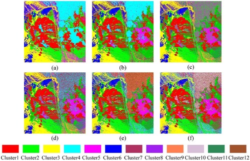
Table 4. Eigenvector selection results and corresponding mapping accuracies of CDMR with different $K$ values.

	CDMR-ARI						CDMR-AMI
K	6	8	9	10	11	12	6	8	9	10	11	12
Band1	5	5	5	5	5	5	5	5	5	5	5	5
Band2	3	3	3	3	3	3	3	3	3	3	3	3
Band3	9	9	9	9	9	9	9	9	9	9	9	9
Band4	10	10	10	14	14	14	10	10	10	10	10	10
Band5	8	14	14	10	10	10	14	14	14	14	14	14
Band6	14	\	\	\	\	\	13	15	15	\	\	\
OA	0.84	0.86	0.86	0.86	0.86	0.86	0.83	0.85	0.85	0.86	0.86	0.86
KC	0.80	0.82	0.82	0.82	0.82	0.82	0.78	0.81	0.81	0.82	0.82	0.82

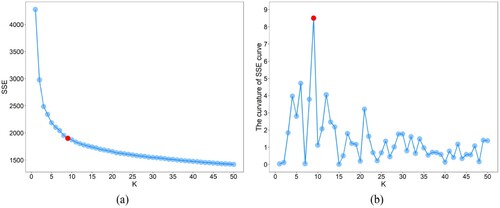
Figure 13. SSE (a) and curvature (b) curves of the AVIRIS image. The red dot represents the point with the maximum curvature.

Data availability statement

The data that support the findings of this study are openly available in https://www.ehu.eus/ccwintco/index.php?title=Hyperspectral_Remote_Sensing_Scenes.