Local climate zone mapping using remote sensing: a synergetic use of daytime multi-view Ziyuan-3 stereo imageries and Luojia-1 nighttime light data

Figures & data

Figure 1. Overview of the study area: (a) the geographic location of the study area; (b) ZY-3 true-color composited image; (c) Luojia-1 nighttime light image; and (d) road networks.

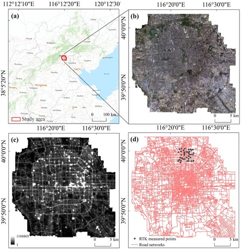
Table 1. Satellite parameters of ZY-3 and Luojia-1 imageries (note that PAN refers to panchromatic and MS multi-spectral).

Parameter	ZY-3	Luojia-1
Launch time	09 January, 2012	02 June, 2018
Orbit altitude (km)	506	634
Swath width (km)	51 × 51	260 × 260
Spatial resolution (m)	PAN-nadir: 2.1 PAN-forward: 3.5 PAN-backward: 3.5 MS: 5.8 Pan-sharpened fusion: 2	130
Wavelength (nm)	PAN band: 500–800 Red band: 630–690 Green band: 520–590 Blue band: 450–520 Near-Infrared band: 770–890	480–800

Figure 2. Proposed workflow of the LCZ mapping.

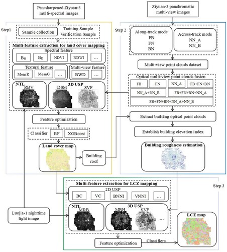
Table 2. Multi-feature extraction for land cover mapping.

Category	Feature	Description/formula	References
Spectral feature	Spectral information	Red band (BR), green band (BG), blue band (BB), and near-infrared band (BNIR)	Faridatul and Wu (2018)
	Normalized Difference Vegetation Index (NDVI)	NDVI = (BNIR− BR)/ (BNIR + BR)	Jiang et al. (2006)
	Ratio Vegetation Index (RVI)	RVI = BNIR/BR	Priebe et al. (1999)
	Difference Vegetation Index (DVI)	DVI = BNIR − BR	Tucker (1979)
	Normalized Difference Water Index (NDWI)	NDWI = (BNIR− BG)/ (BNIR + BG)	McFeeters (1996)
	Morphological Building Index (MBI)	MBI was used to extract buildings by establishing the relationship between implicit features and morphological operators of facilities.	Huang and Zhang (2011)
	Morphological Shadow Index (MSI)	MSI is defined as a dual function of MBI, which highlights the shadow structure.	Huang and Zhang (2012)
Textural feature	Meani	The mean derived from GLCM (note that i refers to different spectral bands).	Huang and Wang (2019)
	Variancei	The variance was derived from GLCM.
	Homogeneityi	The homogeneity was derived from GLCM.
	Contrasti	The contrast was derived from GLCM.
	Dissimilarityi	The heterogeneity parameters were derived from GLCM.	Shaban and Dikshit (2001)
	Entropyi	The entropy was derived from GLCM.	Anys et al. (1998)
	Angular Second Momenti	The angular second moment was derived from GLCM.	Kim et al. (2011)
	Correlationi	The gray correlation was derived from GLCM.	Shafiq et al. (2015)
Multi-view feature	Nadir view (NAD)	A nadir panchromatic band resample to the spatial resolution of 2-m.	Huang et al. (2021)
	Forward view (FWD)	A forward panchromatic band resample to the spatial resolution of 2-m.
	Backward view (BWD)	A backward panchromatic band resamples to the spatial resolution of 2-m.
3D USP	Digital Surface Model (DSM)	The digital surface model is a ground elevation model that includes surface buildings, bridges, trees, etc.	Gomez, Hayakawa, and Obanawa (2015)
	Sky View Factor (SVF)	The sky view factor refers to the visible degree of the sky at the ground level. Its values vary from 0 to 1 and refer to the sky as not visible; in contrast, one refers to the evident atmosphere.	Zakšek, Oštir, and Kokalj (2011)
NTL	Radiation Brightness Value (RBV)	The radiation brightness value is the most intuitive feature of nighttime light images.	Huang et al. (2021)

Table 3. Multi-feature extraction for LCZ mapping.

Category	Feature	Description/formula	References
2D USP	Building coverage (BC)	The total building area is divided by the corresponding LCZ area.	Chen, Xu, and Devereux (2014)
	Vegetation coverage (VC)	The total vegetation area is divided by the corresponding LCZ area.	Cao et al. (2020b)
	Soil coverage (SC)	The total soil area is divided by the corresponding LCZ area.	Sanlang et al. (2021)
	Impervious surface coverage (ISC)	The total impervious surface coverage is divided by the corresponding LCZ area.	Homer et al. (2020)
	Water coverage (WC)	The total water area is divided by the corresponding LCZ area.	Sanlang et al. (2021)
	Building nearest neighbor index (BNNI)	The Nearest Neighbor Index (NNI) value of buildings.	Zhang, Du, and Wang (2018)
	Vegetation nearest neighbor index (VNNI)	The NNI value of vegetation.
	Soil nearest neighbor index (SNNI)	The NNI value of soil lands.
	Impervious nearest neighbor index (INNI)	The NNI value of impervious surfaces.
	Water nearest neighbor index (WNNI)	The NNI value of water bodies.
3D USP	Mean building height (MBH)	The average value of building heights in a LCZ unit.	Li et al. (2020)
	Mean building volume (MBV)	The average value of building volumes in a LCZ unit.
	Mean street width (MSW)	Average street width in a block unit.	Hermosilla et al. (2014)
	Sky view factor (SVF)	Sky view factor influenced by building.	Zakšek, Oštir, and Kokalj (2011)
	Canyon aspect ratio (CAR)	Average canyon height divided street width.	Chen, Xu, and Devereux (2014)
	Floor area ratio (FAR)	Total building area divided by block size.	Hermosilla et al. (2014)
	Frontal area index (FAI)	The frontal area divided the area of the block unit.	Kanda, Kawai, and Nakagawa (2005)
NTL	Mean radiation brightness (MRB)	Average brightness in a block unit.	Huang et al. (2021)

Table 4. Experiments used for LCZ mapping.

Experiment	2D USP	3D USP	NTL
Exp. a	√
Exp. b		√
Exp. c			√
Exp. d	√	√
Exp. e	√		√
Exp. f		√	√
Exp. g	√	√	√

Figure 3. Variable importance ranking for land cover mapping revealed by the RF algorithm.

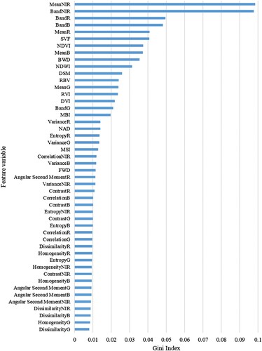
Table 5. Comparison of the performances of RF and XGBoost algorithms in land cover mapping. Note that the kappa coefficient, OA, PA, and UA represent a measure of classification accuracy, overall accuracy, producer’s accuracy, and user’s accuracy, respectively.

Category	RF (%)		XGBoost (%)
	PA	UA	PA	UA
Building	96.79	98.33	96.00	97.43
Vegetation	97.74	96.03	96.73	93.18
Soil	96.20	94.16	90.31	86.91
Impervious ground	94.14	93.69	88.76	90.97
Water	95.48	99.20	94.08	99.02
OA	96.56		94.70
Kappa coefficient	94.73		91.84

Figure 4. Comparison of classification details by using the two classifiers: (a) RF classifier, (b) XGBoost classifier, (c) regions of interest c, (d) regions of interest d. Building outlines, vegetation information and water bodies, and human editing processes produced the comprehensive ‘reference model’.

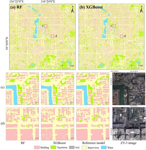
Figure 5. Characteristics of ZY-3 along- and across-track point clouds: (a) NN_A (nadir01 + nadir02), (b) FB (forward + backward), (c) FN (forward + nadir01), (d) false-color composite image, and (e) the number of multi-view point clouds in different land covers.

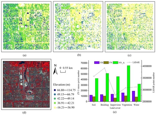
Table 6. Changes in R² value, RMSE value, and building number under varying threshold settings.

Threshold value	R^2 value	RMSE value	Building number
0	0.12	20.79	3070
1	0.52	12.69	2972
2	0.56	11.92	2937
3	0.61	11.16	2904
4	0.65	10.37	2872
5	0.71	9.69	2844
6	0.72	9.22	2810
7	0.73	9.06	2782
8	0.75	8.70	2745
9	0.76	8.56	2727
10	0.76	8.43	2691

Figure 6. Building roughness estimation.

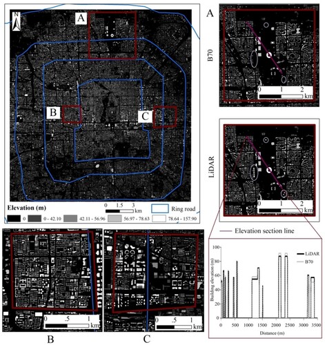
Figure 7. Variable importance ranking for LCZ mapping revealed by the RF algorithm.

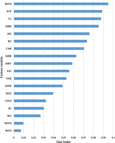
Table 7. A comparison of using RF and XGBoost algorithms in LCZ mapping.

Category	RF (%)		XGBoost (%)
	PA	UA	PA	UA
1	89.47	100.00	89.47	94.44
2	83.67	95.35	79.59	95.12
3	81.82	100.00	78.79	96.30
4	93.58	91.62	91.44	88.60
5	93.55	93.05	94.62	89.80
6	84.13	86.89	80.95	87.93
7	100.00	100.00	84.62	84.62
8	88.24	83.33	85.29	80.56
9	90.59	86.52	88.24	86.21
A	100.00	89.83	86.79	88.46
C	100.00	100.00	90.00	81.82
D	93.88	90.20	93.88	92.00
E	95.33	86.81	93.46	86.06
F	82.89	88.73	85.53	86.67
G	85.29	100.00	88.24	100.00
OA	90.46		88.82
Kappa	89.41		87.59

Figure 8. Comparison of classification details by using the two classifiers. (a) RF classifier-study area, (b) XGBoost classifier-study area, (c) regions of interest c, (d) regions of interest d.

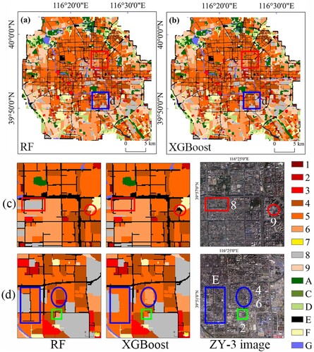
Table 8. Comparison of land cover classification accuracy using the RF classifier and different feature combinations.

Category	PA value (%)
	2D USP + 3D USP (produced by along- and across-track modes) + NTL (Experiment 1)	2D USP + 3D USP (produced by single along-track mode) + NTL (Experiment 2)	2D USP + 3D USP (produced by along- and across- track modes) (Experiment 3)
Building	96.79	90.81	93.66
Vegetation	97.74	93.52	93.01
Soil	96.20	93.09	90.97
Impervious surface	94.14	91.54	90.14
Water	95.48	92.68	92.06
OA	96.56	91.90	92.74
Kappa	94.73	87.65	88.87

Figure 9. Three representative examples of classification details used 2D USP + 3D USP (produced by along- and across-track modes) + NTL, 2D USP + 3D USP (produced by single along-track mode) + NTL, and 2D USP + 3D USP (produced by along- and across-track modes).

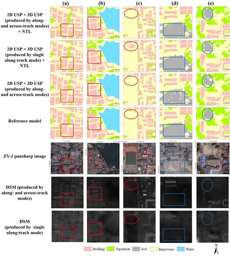
Figure 10. Comparisons of the LCZ classification results of different experiments. Exp. a is the classification experiment without 3D USPs and NTL, Exps. d and e are the classification experiments without NTL and 3D USPs. Exp. g is the classification experiment using 3D USPs and NTL.

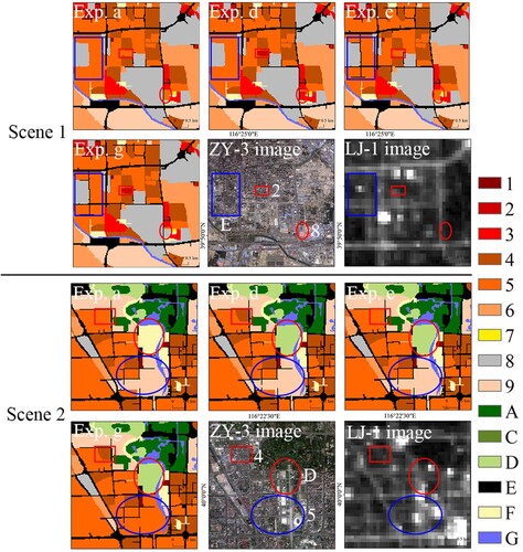
Table 9. Comparisons of the existing methods for LCZ mapping.

Method	Data source	Study area	OA Value
LCZNet (Liu and Shi 2020)	Sentinel-2 multi-spectral data (10 m)	Greater Bay Area, Shanghai Metropolis, and Beijing Metropolis	88.61%
Supervised CNNs (Rosentreter, Hagensieker, and Waske 2020)	Multi-temporal Sentinel-2 composites	Eight German cities	86.50%
Semi-automatic algorithm (Chen, Zheng, and Hu 2020)	Landsat-8 remote sensing images (15 m), building data, and land use data	Chenzhou, China	69.54%
Canonical correlation forest (CCF) (Hu, Ghamisi, and Zhu 2018)	Sentinel-1 dual-pol data (10 m)	29 cities on a global scale	61.8%
Random forest classifier (Chen et al. 2021)	Sentinel-2 multispectral imagery and dual-polarized (HH + HV) PALSAR-2 data	Nanchang, China	89.96%
Residual convolutional neural Network (ResNet) (Qiu et al. 2018)	Sentinel-2 and Landsat-8 imagery, and the VIIRS-based NTL data	nine cities in Europe	78%
WUDAPT level 0 method (Wang et al. 2018)	Landsat-5 satellite images (30 m)	Hong Kong, China	58.00%
Proposed method	ZY-3 images 2.1 m resolution and Luojia-1 image 130 m resolution	Beijing, China	90.46%

Faridatul, M. I., and B. Wu. 2018. “Automatic Classification of Major Urban Land Covers Based on Novel Spectral Indices.” ISPRS International Journal of Geo-Information 7 (12). https://doi.org/10.3390/ijgi7120453.

 PubMed Web of Science ®Google Scholar

Jiang, Z., A. R. Huete, J. Chen, Y. Chen, J. Li, G. Yan, and X. Zhang. 2006. “Analysis of NDVI and Scaled Difference Vegetation Index Retrievals of Vegetation Fraction.” Remote Sensing of Environment 101 (3): 366–378. https://doi.org/10.1016/j.rse.2006.01.003.

 Web of Science ®Google Scholar

Priebe, S., P. Huxley, S. Knight, and S.E. Summary. 1999. “Application and Results of the Manchester Short Assessment of Quality of Life (Mansa) Background Based on Experiences and Empirical Evidence Gained in Studies Using the Lancashire Quality of Life Profile (LQLP), the Manchester Short.” 7–12.

 Google Scholar

Tucker, C.J. 1979. “Red and Photographic Infrared Linear Combinations for Monitoring Vegetation.” Remote Sensing of Environment 8 (2): 127–150. https://doi.org/10.1016/0034-4257(79)90013-0.

 Web of Science ®Google Scholar

McFeeters, S. K. 1996. “The Use of the Normalized Difference Water Index (NDWI) in the Delineation of Open Water Features.” International Journal of Remote Sensing 17 (7): 1425–1432. https://doi.org/10.1080/01431169608948714.

 Web of Science ®Google Scholar

Huang, X., and L. Zhang. 2011. “A Multidirectional and Multiscale Morphological Index for Automatic Building Extraction from Multispectral GeoEye-1 Imagery” Photogrammetric Engineering & Remote Sensing 77 (7): 721–732. https://doi.org/10.14358/PERS.77.7.721.

 Web of Science ®Google Scholar

Huang, X., and L. Zhang. 2012. “Morphological Building/Shadow Index for Building Extraction from High-Resolution Imagery Over Urban Areas.” IEEE Journal of Selected Topics in Applied Earth Observations and Remote Sensing 5 (1): 161–172. https://doi.org/10.1109/JSTARS.2011.2168195.

 Web of Science ®Google Scholar

Huang, X., and Y. Wang. 2019. “Investigating the Effects of 3D Urban Morphology on the Surface Urban Heat Island Effect in Urban Functional Zones by Using High-Resolution Remote Sensing Data: A Case Study of Wuhan, Central China.” ISPRS Journal of Photogrammetry and Remote Sensing 152:119–131. https://doi.org/10.1016/j.isprsjprs.2019.04.010.

 Web of Science ®Google Scholar

Shaban, M. A., and O. Dikshit. 2001. “Improvement of Classification in Urban Areas by the Use of Textural Features: The Case Study of Lucknow City, Uttar Pradesh.” International Journal of Remote Sensing 22 (4): 565–593. https://doi.org/10.1080/01431160050505865.

 Web of Science ®Google Scholar

Anys, H., A. Bannari, D. C. He, and D. Morin. 1998. “Cartographie des Zones Urbaines a L'aide des Images Aeroportees MEIS-II” International Journal of Remote Sensing 19 (5): 883–894. https://doi.org/10.1080/014311698215775.

 Web of Science ®Google Scholar

Kim, M., T. A. Warner, M. Madden, and D. S. Atkinson. 2011. “Multi-Scale GEOBIA with Very High Spatial Resolution Digital Aerial Imagery: Scale, Texture and Image Objects.” International Journal of Remote Sensing 32 (10): 2825–2850. https://doi.org/10.1080/01431161003745608.

 Web of Science ®Google Scholar

Shafiq, M. A., Z. Wang, A. Amin, T. Hegazy, M. Deriche, and G. AlRegib. 2015. “Detection of Salt-Dome Boundary Surfaces in Migrated Seismic Volumes Using Gradient of Textures.” SEG Technical Program Expanded Abstracts 34:1811–1815. https://doi.org/10.1190/segam2015-5927230.1.

 Google Scholar

Huang, X., J. Yang, J. Li, and D. Wen. 2021. “Urban Functional Zone Mapping by Integrating High Spatial Resolution Nighttime Light and Daytime Multi-View Imagery.” ISPRS Journal of Photogrammetry and Remote Sensing 175:403–415. https://doi.org/10.1016/j.isprsjprs.2021.03.019.

 Web of Science ®Google Scholar

Gomez, C., Y. Hayakawa, and H. Obanawa. 2015. “A Study of Japanese Landscapes Using Structure from Motion Derived DSMs and DEMs Based on Historical Aerial Photographs: New Opportunities for Vegetation Monitoring and Diachronic Geomorphology.” Geomorphology 242:11–20. https://doi.org/10.1016/j.geomorph.2015.02.021.

 Web of Science ®Google Scholar

Zakšek, K., K. Oštir, and Ž. Kokalj. 2011. “Sky-View Factor as a Relief Visualization Technique.” Remote Sensing 3 (2): 398–415. https://doi.org/10.3390/rs3020398.

 Web of Science ®Google Scholar

Chen, Z., B. Xu, and B. Devereux. 2014. “Urban Landscape Pattern Analysis Based on 3D Landscape Models.” Applied Geography 55: 82–91. https://doi.org/10.1016/j.apgeog.2014.09.006.

 Web of Science ®Google Scholar

Cao, S., Q. Weng, M. Du, B. Li, R. Zhong, and Y. Mo. 2020b. “Multi-scale Three-Dimensional Detection of Urban Buildings Using Aerial LiDAR Data.” GIScience & Remote Sensing 57 (8): 1125–1143. https://doi.org/10.1080/15481603.2020.1847453.

 Web of Science ®Google Scholar

Sanlang, S., S. Cao, M. Du, Y. Mo, Q. Chen, and W. He. 2021. “Integrating Aerial Lidar and Very-High-Resolution Images for Urban Functional Zone Mapping.” Remote Sensing 13 (13). https://doi.org/10.3390/rs13132573.

 Web of Science ®Google Scholar

Homer, C., J. Dewitz, S. Jin, G. Xian, C. Costello, P. Danielson, L. Gass, et al. 2020. “Conterminous United States Land Cover Change Patterns 2001–2016 from the 2016 National Land Cover Database.” ISPRS Journal of Photogrammetry and Remote Sensing 162:184–199. https://doi.org/10.1016/j.isprsjprs.2020.02.019.

 PubMed Web of Science ®Google Scholar

Zhang, X., S. Du, and Q. Wang. 2018. “Integrating Bottom-up Classification and Top-Down Feedback for Improving Urban Land-Cover and Functional-Zone Mapping.” Remote Sensing of Environment 212:231–248. https://doi.org/10.1016/j.rse.2018.05.006.

 Web of Science ®Google Scholar

Li, M., E. Koks, H. Taubenböck, and J. van Vliet. 2020. “Continental-Scale Mapping and Analysis of 3D Building Structure.” Remote Sensing of Environment 245:111859. https://doi.org/10.1016/j.rse.2020.111859.

 Web of Science ®Google Scholar

Hermosilla, T., J. Palomar-Vázquez, Á Balaguer-Beser, J. Balsa-Barreiro, and L. A. Ruiz. 2014. “Using Street Based Metrics to Characterize Urban Typologies.” Computers, Environment and Urban Systems 44:68–79. https://doi.org/10.1016/j.compenvurbsys.2013.12.002.

 Web of Science ®Google Scholar

Kanda, M., T. Kawai, and K. Nakagawa. 2005. “A Simple Theoretical Radiation Scheme for Regular Building Arrays.” Boundary-Layer Meteorology 114 (1): 71–90. https://doi.org/10.1007/s10546-004-8662-4.

 Web of Science ®Google Scholar

Liu, S., and Q. Shi. 2020. “Local Climate Zone Mapping as Remote Sensing Scene Classification Using Deep Learning: A Case Study of Metropolitan China.” ISPRS Journal of Photogrammetry and Remote Sensing 164:229–242. https://doi.org/10.1016/j.isprsjprs.2020.04.008.

 Web of Science ®Google Scholar

Rosentreter, J., R. Hagensieker, and B. Waske. 2020. “Towards Large-Scale Mapping of Local Climate Zones Using Multitemporal Sentinel 2 Data and Convolutional Neural Networks.” Remote Sensing of Environment 237:111472. https://doi.org/10.1016/j.rse.2019.111472.

 Web of Science ®Google Scholar

Chen, Y., B. Zheng, and Y. Hu. 2020. “Mapping Local Climate Zones Using arcGIS-Based Method and Exploring Land Surface Temperature Characteristics in Chenzhou, China.” Sustainability 12 (7). https://doi.org/10.3390/su12072974.

 Web of Science ®Google Scholar

Hu, J., P. Ghamisi, and X. X. Zhu. 2018. “Feature Extraction and Selection of Sentinel-1 Dual-Pol Data for Global-Scale Local Climate Zone Classification.” ISPRS International Journal of Geo-Information 7 (9): 1–20. https://doi.org/10.3390/ijgi7090379.

 Web of Science ®Google Scholar

Chen, C., H. Bagan, X. Xie, Y. La, and Y. Yamagata. 2021. “Combination of Sentinel-2 and Palsar-2 for Local Climate Zone Classification: A Case Study of Nanchang, China.” Remote Sensing 13 (10): 1–21. https://doi.org/10.3390/rs13101902.

 PubMed Web of Science ®Google Scholar

Qiu, C., M. Schmitt, L. Mou, P. Ghamisi, and X. X. Zhu. 2018. “Feature Importance Analysis for Local Climate Zone Classification Using a Residual Convolutional Neural Network with Multi-Source Datasets.” Remote Sensing 10 (10): 1–14. https://doi.org/10.3390/rs10101572.

 Web of Science ®Google Scholar

Wang, R., C. Ren, Y. Xu, K. K. L. Lau, and Y. Shi. 2018. “Mapping the Local Climate Zones of Urban Areas by GIS-Based and WUDAPT Methods: A Case Study of Hong Kong.” Urban Climate 24:567–576. https://doi.org/10.1016/j.uclim.2017.10.001.

 Web of Science ®Google Scholar

Data availability statement

The data that support the findings of this study are available from the corresponding author upon reasonable request. Data in this study can be available within the article or its supplementary materials.