
Figures & data
Figure 1. Spatio-temporal representational learning.
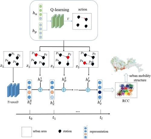
Figure 2. Policy design.
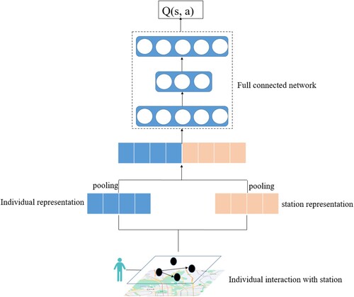
Figure 3. Robust continuous clustering process.
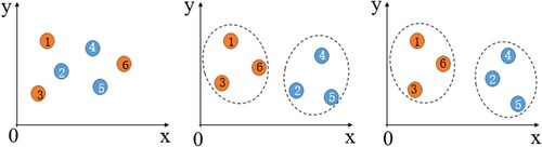
Figure 4. Study area.
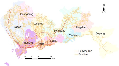
Table 1. Example of passenger travel chain for April 3, 2017.
Table 2. Data description.
Figure 5. Results on weekdays and weekends. (a) Weekdays. (b) Weekends.
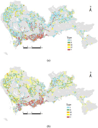
Figure 6. Statistical results. (a) Average travel time (b) Average stay time (c) Average travel distance (d) Distance to the nearest bus stop.
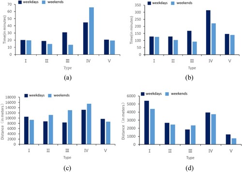
Figure 7. Flow between types (The size of the circle indicates the area of the urban mobility structure, the color indicates different types of urban mobility structures consistent with , the statistical map inside the circle indicates the normalized value of the density of each type of POI, the direction of the arrow indicates the flow direction, and the thickness of the arrow indicates the flow size) (a) weekdays (b) weekends.

Figure 8. Morning and evening peak urban mobility structure map (a) morning peak (b) evening peak.
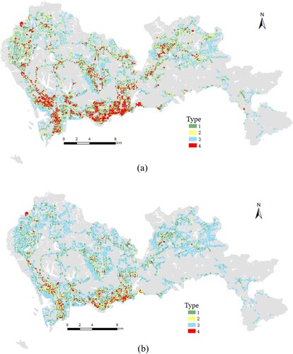
Figure 9. Comparison of the algorithm's urban mobility structure on weekdays (a) Combo (b) GraphEncoder (c) Joint embedding (d) Ablation study.
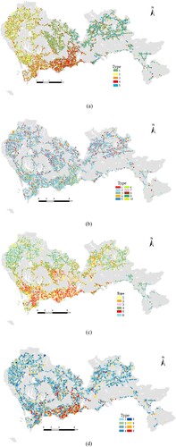
Table 3. Comparison of Q-value of various methods.
Figure 10. Visualization results of T-SNE algorithm (a) Combo (b) GraphEncoder (c) Group-based integrated representational learning (d) Ablation study (e) Our method.
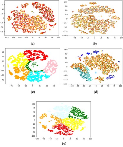
Figure 11. Parameter sensitivity results (a) Precision on Station ID (b) Average Similarity.
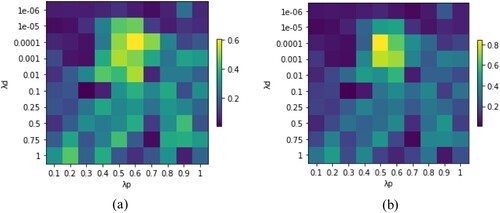
Table 4. Comparison on Precision on Station ID and Distance similarity.