Estimating daily surface downward shortwave radiation over rugged terrain without bright surface at 30 m on clear-sky days using CERES data

Figures & data

Figure 1. Spatial distribution of the six mountainous sites: (a) All sites over the globe. (b) One site, GMN-PG3, in the Sierra Nevada in Spain, and (c) The other five sites (sites 2–4 and site 6–7) in the Chengde Experimental Area. The legend in (a) represents the classes of mountains as defined by the United Nations Environment Program World Conservation Monitoring Center (UNEP-WCMC), and the legends in (b) and (c) show the elevations obtained from the Shuttle Radar Topography Mission (SRTM).

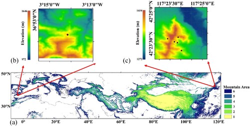
Table 1. Detailed information of the six sites used in this study.

Site Name	Latitude (°)	Longitude(°)	Elevation (m)	S * (°)	A * (°)
site2	42.397	117.398	1848.427	19	269
site3	42.393	117.397	1852.700	26	196
site4	42.393	117.395	1810.066	22	285
site6	42.396	117.390	1756.811	29	189
site7	42.387	117.400	1838.169	30	138
GMN-PG3	36.872	−3.236	1332	20.81	15.26

*S and A represent slope and aspect.

Figure 2. The different ways to deploy the measuring instrument on a sloped surface: (a) parallel to the horizontal surface, (b) parallel to the inclined surface, and (c) diagram of the corresponding θ_i and solar zenith angle θ₀.

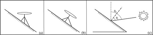
Figure 3. Diagram of calculation of factors of the terrain of the target pixel Z₅. Z represents the elevation of the pixel.

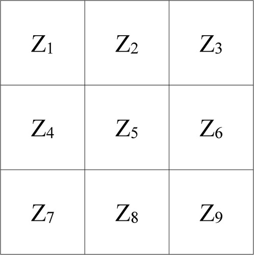
Table 2. Classes of Mountains defined in UNEP-WCMC.

Class (elevation in meters)	Additional Criterion	% of the Earth's Surface
>4,500		1.2
3,500 ∼ 4,499		1.8
2,500 ∼ 3,499		4.7
1,500 ∼ 2,499	S > 2°	3.6
1,000 ∼ 1,499	S > 5° or LER > 300m	4.2
300 ∼ 999	LER > 300m	8.8
Total		24.3

LER (Local Elevation Range) represents the elevation range in an area assessing over a seven-mile radius.

Figure 4. The flowchart of this study.

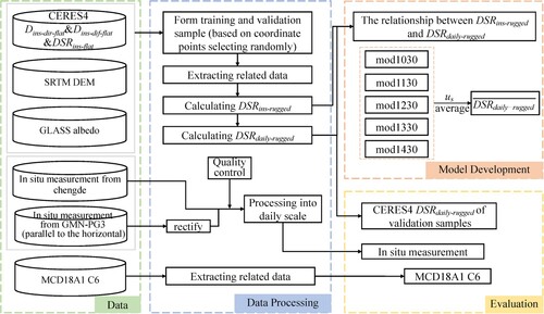
Figure 5. Schematic diagram of determining whether a pixel was blocked by neighboring pixels.

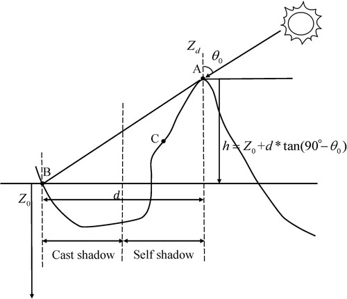
Figure 6. The structure of random forest regression.

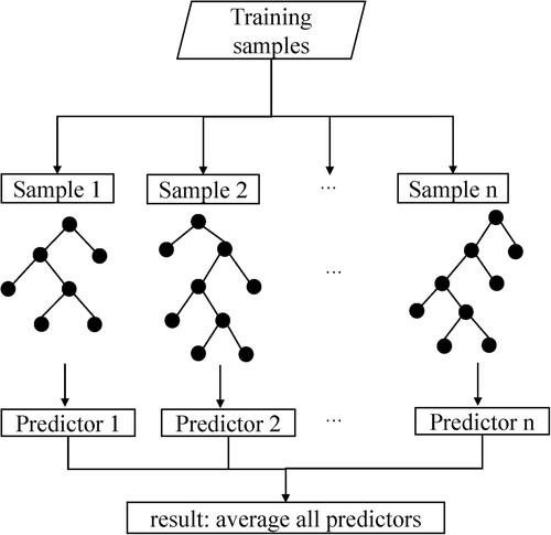
Figure 7. Spatial distributions of (a) the 17 study regions within typical mountainous areas (see Table 2) across the world, and the training and validation samples acquired from them (a1)–(a17). The legend in (a) represents the classes of mountains and that in (b) represents the land cover type as defined by the International Geosphere–Biosphere Program (IGBP) based on MCD12 C1 in 2015.

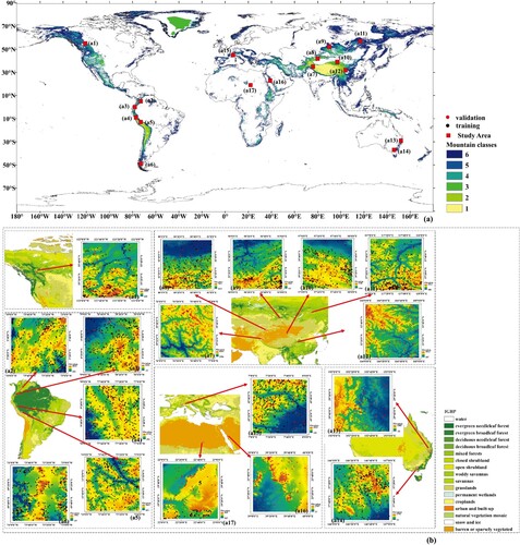
Figure 8. The statistics on all training (orange bar) and validation samples (yellow bar) of DSR_daily-rugged based on various factors: (a) A (0−360°) with an interval of 45°, (b) S (0−90°) with an interval of 10°, (c) φ (latitude) within 40° S−90° S, 20° S−40° S, 0°−20° S, 0°−20° N, 20°−40° N, and 40°−90° N, (d) V_d (0.5∼1) with an interval of 0.1, (e) doy (1∼365) with an interval of 60, and (f) elevation as determined by the six mountain classes defined in Table 2.

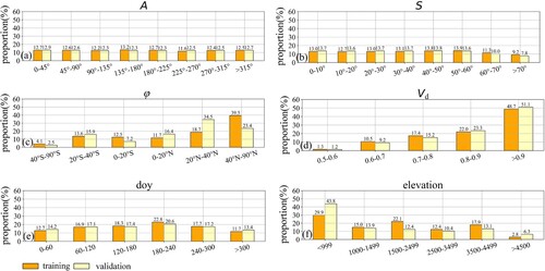
Figure 9. Scatter plots between DSR_ins-rugged and DSR_daily-rugged at (a) 8:30, (b) 9:30, (c) 10:30, (d) 11:30, (e) 12:30, (f) 13:30, (g) 14:30, (h) 15:30, (i) 16:30, and (j)17:30hrs, local time.

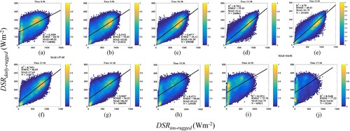
Figure 10. The correlation between DSR_ins-rugged and DSR_daily-rugged as represented by R² under different combinations of S and A at five times: (a) 10:30, (b) 11:30, (c) 12:30, (d) 13:30, and (e) 14:30hrs. (f) The corresponding sample size at the five times, and the different colors indicate the numbers of different samples.

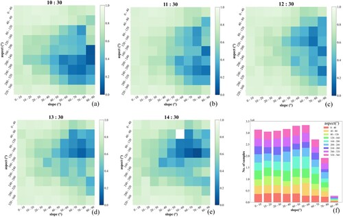
Figure 11. The relationship between DSR_{daily−rugged} and DSR_daily−flat as represented by the normalized RMSE, normalized MAE obtained by normalizing the original RMSE and the MAE through min-max normalization method for clearer presentation, and R² with different slopes. The closer R² to zero, and close the normalized RMSE and the MAE were to one, the worse was the correlation, and vice versa.

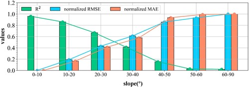
Table 3. The relationship between DSR_ins-rugged and DSR_daily-rugged as represented by the RMSE and R² for different albedo values at an interval of 0.2 from 0−0.7 at five times (10:30, 11:30, 12:30, 13:30, and 14:30hrs).

albedo	10:30	11:30	12:30	13:30	14:30
RMSE (Wm^−2)
0 − 0.2	45.16	39.13	40.02	46.89	56.67
0.2 − 0.4	43.73	37.33	38.64	44.97	53.83
0.4 − 0.6	43.40	41.53	43.80	47.97	56.80
0.6 − 0.7	51.08	47.31	47.42	50.16	58.68
R^2
0 − 0.2	0.70	0.78	0.78	0.70	0.56
0.2 − 0.4	0.70	0.79	0.78	0.70	0.53
0.4 − 0.6	0.75	0.80	0.76	0.72	0.60
0.6 − 0.7	0.64	0.70	0.70	0.67	0.57

Table 4. Hyper-parameter settings used to identify five optimal DSRMT models. The three values in brackets for each hyper-parameter of every model represent the start, interval, and end values, respectively, and the values in parentheses represent the value of the confirming hyper-parameter.

	Hyper-Parameters
	n-estimators	max depth	min samples split	min samples leaf
mod1030	[30,10,70] (40)	[10,5,40] (20)	[2, 2,10] (2)	[2,2, 10] (4)
mod1130	[30,10,70] (60)	[10,5,40] (15)	[2, 2,10] (2)	[2,2, 10] (8)
mod1230	[30,10,70] (60)	[10,5,40] (15)	[2, 2,10] (2)	[2,2, 10] (8)
mod1330	[30,10,70] (40)	[10,5,40] (15)	[2, 2,10] (2)	[2,2, 10] (8)
mod1430	[30,10,70] (40)	[10,5,40] (15)	[2, 2,10] (2)	[2,2, 10] (8)

Figure 12. The overall accuracy of the $\overline{\mathrm{DS}{\mathrm{R}}_{\mathrm{daily}\text{-}\mathrm{rugged}}}$, obtained by the weighted average of the outputs of the five DSRMT models based on all training samples.

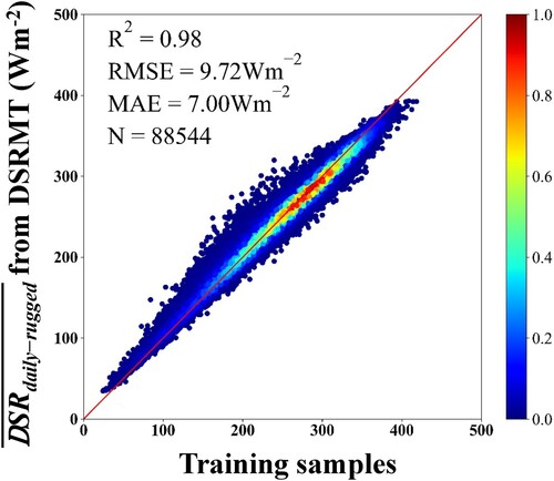
Table 5. The accuracy of validation of the five DSRMT models using validation samples from CERES4.

Model	Validation accuracy			No. of samples
	RMSE (Wm^−2)	MAE (Wm^−2)	R^2
mod1030	19.51	14.82	0.90	86,733
mod1130	18.17	13.70	0.91	86,733
mod1230	17.41	13.10	0.92	86,733
mod1330	19.82	15.10	0.89	86,733
mod1430	22.67	17.31	0.86	86,733

Figure 13. The accuracy of validation of $\overline{\mathrm{DS}{\mathrm{R}}_{\mathrm{daily}\text{-}\mathrm{rugged}}}$ based on the weighted average of five DSR_daily-rugged estimates of the five DSRMT models by using (a) all validation samples from CERES4, (b) validation samples from CERES4 for regions that provided the training samples, and (c) validation samples from CERES4 for regions from which training samples were not chosen.

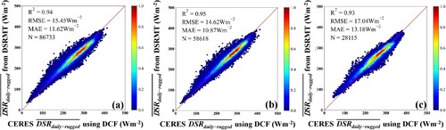
Table 6. The accuracy of validation of $\overline{\mathrm{DS}{\mathrm{R}}_{\mathrm{daily}\text{-}\mathrm{rugged}}}$ calculated by using different combinations of the five DSR_{daily−rugged} estimates from the DSRMT models from 10:30–14:30hrs based on all validation samples from CERES4. The letters A, B, C, D, and E represents the DSR_{daily−rugged} estimates of mod1030, mod1130, mod1230, mod1330, and mod1430, respectively.

Combinations	RMSE (Wm^−2)	MAE (Wm^−2)	R^2	combinations	RMSE (Wm^−2)	MAE (Wm^−2)	R^2
A – E	15.45	11.62	0.94	A, B, E	15.89	11.96	0.94
A, B	17.28	13.16	0.92	A, C, D	15.61	11.71	0.94
A, C	16.04	12.06	0.93	A, C, E	15.70	11.79	0.94
A, D	16.32	12.23	0.93	A, D, E	16.51	12.50	0.93
A, E	16.88	12.68	0.93	B, C, D	15.99	12.04	0.93
B, C	16.27	12.24	0.93	B, C, E	16.10	12.16	0.93
B, D	16.49	12.41	0.93	B, D, E	16.85	12.83	0.93
B, E	16.96	12.84	0.93	C, D, E	17.60	13.46	0.92
C, D	17.17	13.04	0.92	A, B, C, D	15.40	11.55	0.94
C, E	17.68	13.49	0.92	A, B, C, E	15.39	11.55	0.94
D, E	19.78	15.20	0.90	A, B, D, E	15.74	11.85	0.94
A, B, C	15.87	11.98	0.93	A, C, D, E	15.86	11.98	0.94
A, B, D	15.75	11.83	0.94	B, C, D, E	16.25	12.32	0.93

Table 7. Results of validation of the five DSRMT models in terms of estimating DSR_daily-rugged in comparison with in-situ measurements from six mountainous areas.

Model	Validation accuracy
	RMSE (Wm^−2)	MAE (Wm^−2)	R^2
mod1030	26.39	19.28	0.92
mod1130	29.22	22.94	0.92
mod1230	24.90	19.16	0.92
mod1330	25.67	20.82	0.92
mod1430	24.34	20.18	0.91

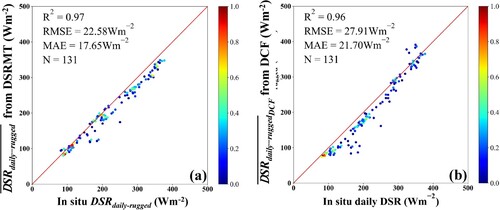
Figure 14. The overall accuracy of validation against in-situ measurements of (a) the optimal $\overline{\mathrm{DS}{\mathrm{R}}_{\mathrm{daily}\text{-}\mathrm{rugged}}}$ estimates according to u_s based on the weighted average of the outputs of the DSRMT models, and (b) ${\overline{\mathrm{DS}{\mathrm{R}}_{\mathrm{daily}\text{-}\mathrm{rugged}}}}_{\mathrm{DCF}}$ estimates obtained by averaging all estimates DSR_ins-rugged by using the DCF method during the day.

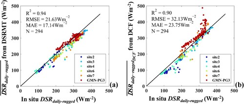
Figure 15. Temporal variations in the values of $\overline{\mathrm{DS}{\mathrm{R}}_{\mathrm{daily}\text{-}\mathrm{rugged}}}$ based on the DSRMT (red line), ${\overline{\mathrm{DS}{\mathrm{R}}_{\mathrm{daily}\text{-}\mathrm{rugged}}}}_{\mathrm{DCF}}$ based on the DCF method (green line), and in-situ measurements (black dot) at (a1) GMN-PG3, (b1) site 2, and (c1) site 4. (a2–a3), (b2–b3), and (c2–c3) show their corresponding scatter plots against the in-situ measurements. Note that the time given on the abscissa is not continuous in (a1)–(c1).

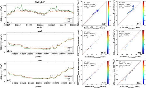
Table 8. The validation results of the sinusoidal method by using data on DSR_ins-rugged from CERES4 at each of the five times as the input against the same in-situ measurements.

Time	Validation accuracy
	RMSE (Wm^−2)	MAE (Wm^−2)	R^2
10:30	45.31	39.24	0.86
11:30	32.10	26.04	0.92
12:30	24.04	17.30	0.94
13:30	28.25	20.35	0.90
14:30	32.96	25.29	0.84

Figure 16. The contributions of all variables of the five DSRMT models.

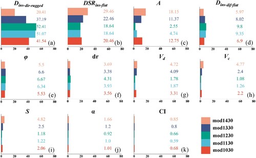
Figure 17. Accuracy of $\overline{\mathrm{DS}{\mathrm{R}}_{\mathrm{daily}\text{-}\mathrm{rugged}}}$ estimates obtained by the DSRMT against in-situ measurements by using DSR-related variables from (a) MCD18 and (b) CERES4 as inputs.

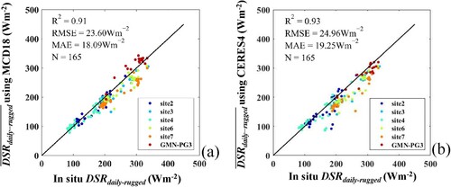
Table 9. The accuracy of validation of estimates of $\overline{\mathrm{DS}{\mathrm{R}}_{\mathrm{daily}\text{-}\mathrm{rugged}}}$ generated by the five DSRMT models under various values of S, A, and elevation.

	RMSE (Wm^−2)	rRMSE (%)	MAE (Wm^−2)	R^2	No. of validation samples
	S
<20°	12.32	4.62	9.40	0.97	17,048
20° − 30°	13.34	5.14	10.21	0.97	17,279
30° − 40°	14.93	5.99	11.47	0.95	16,640
40° − 50°	16.52	6.75	12.51	0.91	14,913
50° − 60°	17.52	7.31	13.29	0.85	12,510
60° − 70°	18.67	8.28	14.39	0.79	5,543
>70°	23.05	10.93	16.98	0.65	2,800
	A
<40°	16.73	7.02	12.79	0.95	9,741
40° − 80°	16.49	6.65	12.96	0.92	7,964
80° − 120°	16.42	6.46	12.01	0.92	8,104
120° − 160°	16.11	6.19	11.79	0.91	10,031
160° − 200°	13.74	5.32	10.7	0.95	10,766
200° − 240°	15.34	6.04	11.27	0.93	12,732
240° − 280°	14.67	5.89	10.78	0.94	8,230
280° − 320°	15.72	6.42	11.86	0.94	9,609
>320°	13.90	5.83	10.74	0.97	9,556
	elevation
<300m	14.25	5.86	11.04	0.96	6,688
300 − 1000m	13.64	5.31	10.40	0.95	42,248
1000 − 1500m	15.87	6.56	12.27	0.95	12,378
1500 − 2500m	17.71	7.13	13.16	0.91	7,446
2500 − 3500m	19.64	8.06	14.51	0.89	5,402
3500 − 4500m	16.58	6.93	12.21	0.93	9,722
>4500m	21.06	8.63	16.55	0.87	2,849

Figure 18. The results of validation based on CERES4 in comparison with in-situ measurements in the presence of shadows. (a) $\overline{\mathrm{DS}{\mathrm{R}}_{\mathrm{daily}\text{-}\mathrm{rugged}}}$ estimates of the proposed model and (b) ${\overline{\mathrm{DS}{\mathrm{R}}_{\mathrm{daily}\text{-}\mathrm{rugged}}}}_{\mathrm{DCF}}$ estimates of the DCF method.