Fractional crop-planting area projection by integrating geographic grid data and agricultural statistics based on random forest regression

Figures & data

Figure 1. Overview of the study area: (a) geographical location; (b) six ecological districts; (c) elevation; (d) land cover and land use.

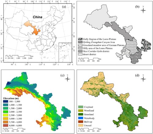
Table 1. Geographic data and agricultural statistics for fractional crop-planting area mapping.

Datasets		Purpose/Variables	Source	Initial Data Declaration
Geographic data	China’s land use and land cover (CNLULC)	Proportion of each 25 land cover classes	Resource and Environmental Science Data Center (http://www.resdc.cn)	100 m
	China’s five-day NDVI composite (MODND1F)	35 NDVI features and 16 phenological features	Geospatial Data Cloud (http://www.gscloud.cn)	500 m, 5 days
	Digital elevation model (DEM) of China	Elevation, slope, and aspect	National Tibetan Plateau Data Center (http://data.tpdc.ac.cn)	1 km
	World Database of Protected Areas (WDPA)	Suitability mask	World Database of Protected Areas (https://www.protectedplanet.net/country/CHN)	shapefile
	China land cover dataset (CLCD)	Independent validation	Zenodo (https://zenodo.org/record/441781)	30 m
Agricultural statistics		Crop-sown areas	Gansu Province Bureau of Statistics (http://tjj.gansu.gov.cn/)	County

Table 2. CNLULC land use classification scheme.

CNLULC Legend
1: Cropland	11: Paddy land		45: Beach and shore
	12: Dry land		46: Bottomland
2: Woodland	21: Forest	5: Unused	51: Urban built-up
	22: Shrub		52: Rural settlements
	23: Woods		53: Other built-up land
	24: Other Woodland	6: Built-up	61: Sandy land
3: Grassland	31: Dense grass		62: Gobi
	32: Moderate grass		63: Salina
	33: Sparse grass		64: Swampland
4: Waterbody	41: Stream and rivers		65: Bare soil
	42: Lakes		66: Bare rock
	43: Reservoir and pond		67: Other unused land
	44: Permanent ice and snow

Figure 2. Workflow of integration of geographic data and agricultural statistics to generate FCPA estimates.

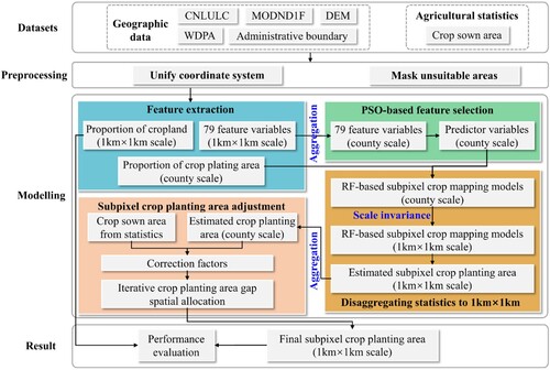
Figure 3. Workflow of adjusting the predicted crop-planting areas by RF models to match the agricultural statistics.

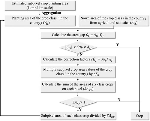
Figure 4. Selected features and their importance ranking: (a)–(f) represents six types of crops (i.e. wheat, maize, oil-bearing, vegetable, orchards, and other crops, respectively).

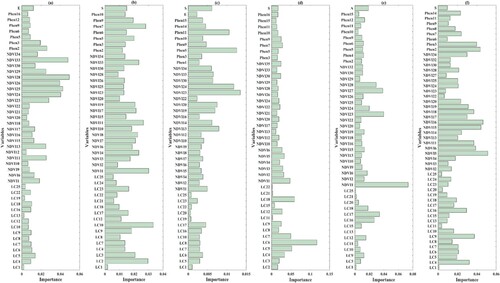
Figure 5. Comparison of agricultural statistics with disaggregating estimates based on RF-based regression models. The first to sixth rows of subplots from top to bottom represent six types of crops (i.e. wheat, maize, oil-bearing, vegetable, orchards, and other crops) respectively. The first to third columns from left to right are (a1–f1) agricultural statistics, and the predicted FCPA by RF models (a2∼f2) without feature selection and (a3∼f3) with PSO feature selection.

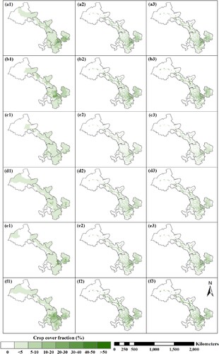
Figure 6. Comparison of agricultural statistics with disaggregating estimates based on adjusted RF regression models. Except for adjusting the prediction of RF-based models, the symbols are identical to those in Figure 5.

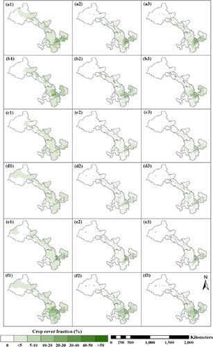
Figure 7. Comparison of agricultural statistics with RF-based downscaled estimates aggregated to the administrative unit level. The first to sixth rows of subplots from top to bottom represented six crops of wheat, maize, oil-bearing, vegetable, orchards, and other crops, respectively. The first to fourth columns from left to right represent downscaled results from ‘RF,’ ‘RF-FS,’ ‘RF-C,’ and ‘RF-FS-C,’ respectively. A red line portrays the 1:1 line for the estimated census relationship and each scatter represents a county.

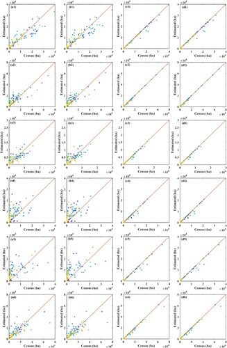
Table 3. Accuracy of the RF-based FCPA mapping models on the county scale.

Metrics	Model	Wheat	Maize	Oil-bearing	Vegetable	Orchards	Other crops
R^2	RF	0.702	0.736	0.579	0.210	0.311	0.588
	RF-FS	0.736	0.759	0.599	0.217	0.334	0.601
	RF-C	0.987	0.998	0.989	0.976	0.982	0.986
	RF-FS-C	0.987	0.998	0.989	0.976	0.982	0.987
RMSE (ha)	RF	4870.50	6584.60	2398.00	6962.60	7350.90	8250.60
	RF-FS	4597.40	6366.00	2400.40	7308.60	7769.80	8082.20
	RF-C	1076.80	503.35	402.25	772.04	1020.30	1693.80
	RF-FS-C	1070.10	506.11	406.16	768.50	1015.00	1619.90
AB (ha)	RF	3202.20	4469.00	1794.90	4851.80	5401.40	4970.30
	RF-FS	3096.00	4430.30	1773.70	4956.40	5784.20	4834.30
	RF-C	285.81	147.42	111.40	211.88	253.24	435.46
	RF-FS-C	280.94	145.04	111.40	208.65	250.82	414.41

Note: In the table, ‘RF’ refers to the RF model that does not consider feature selection, ‘RF-FS’ refers to the RF model that combines PSO feature selection, and RF-C and RF-FS-C, respectively, refer to the postprocessing correction of ‘RF’ and ‘RF-FS.’

Figure 8. Comparison of agricultural statistics of six crops with RF-based downscaled estimates aggregated to the ecological district scale. Each subplot represents an ecological area: (a) hilly area of the Loess Plateau; (b) desert district; (c) Hexi Corridor gobi district; (d) Qinling Zhongshan canyon area; (e) gully region of the Loess Plateau; and (f) grassland meadow area of Gannan Plateau.

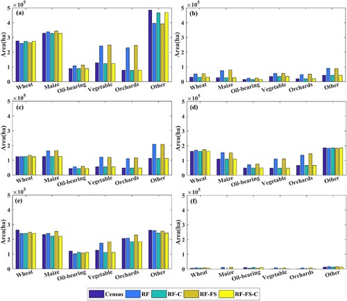
Figure 9. Comparison of cropland distribution from CLCD and estimated total crop-planting area on a 1-km pixel scale: (a) the proportion of cropland calculated using 30-m LCLD data and estimated total crop-planting area by (b) RF, (c) RF-C, (d) RF-FS, and (e) RF-FS-C, respectively.

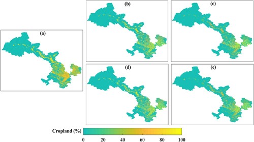
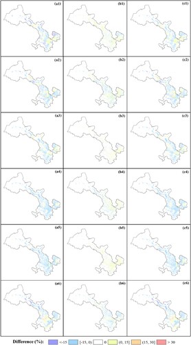
Figure 10. The effect of feature selection and postprocessing adjustment. The first to sixth rows of subplots from top to bottom represent six crops of wheat, maize, oil-bearing, vegetable, orchards, and other crops, respectively. The first to third columns from left to right represent the effects of (a1∼a6) adjustment, (b1∼b6) feature selection, and (c1∼c6) a combination of the two, respectively.

Data availability statement

The data supporting the findings of this study are available from the website provided in the manuscript.