Histogram cube: towards lightweight interactive spatiotemporal aggregation of big earth observation data

Figures & data

Table 1. Types of spatiotemporal aggregation.

Type	Description	Schematic
Temporal Aggregation	Summary statistics along the time dimension
	Example: monthly product from daily vegetation index.
	$⟨S,T⟩\stackrel{group}{\to }⟨S_{zone},T⟩\stackrel{agg}{\to }output$
Spatial Aggregation	Summary of statistics based on space zones
	Example: statistics on the proportion of land use types in administrative regions.
	$⟨S,T⟩\stackrel{group}{\to }⟨S,T_{zone}⟩\stackrel{agg}{\to }output$
Spatiotemporal Independent Aggregation	Statistics by spatiotemporal zones, where space and time are independent of each other
	Example: monthly maximum and minimum land surface temperature for each zone based on daily land surface temperature.
	$⟨S,T⟩\stackrel{group}{\to }⟨S_{zone},T_{zone}⟩\stackrel{agg}{\to }output$
Spatiotemporal Coupled Aggregation	Statistics by spatiotemporal zones, and time zones varies with space zones
	Example: query the rainfall for different crops in the phenological period, where the space zone is the crop distribution area, and the time zone is the phenological period of each crop.
	$⟨S,T⟩\stackrel{group}{\to }⟨S_{zone},T_{zone}⟩\stackrel{agg}{\to }output\wedge T_{zone}=f(S_{zone})$

Figure 1. Conceptual model of the histogram cube.

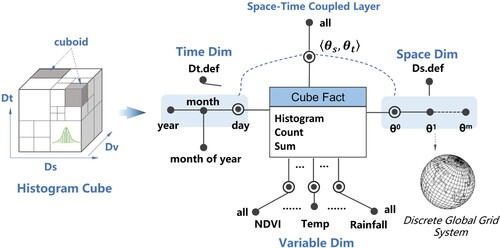
Figure 2. Pyramid structure of histogram cuboids.

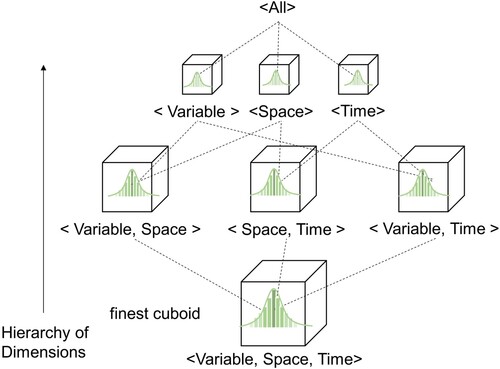
Table 2. Aggregation functions based on a frequency histogram.

Type	Measure	Measure Function	Aggregate Function
Distributive	count	$count=\sum _{i=1}^n{f}_i$	$count=\sum _{i=1}^{n}coun{t}_i$
	sum	$sum=\sum _{i=1}^n{f}_i\ast x_i$	$sum=\sum _{i=1}^{n}su{m}_i$
Algebraic	mean	$mean={\displaystyle \frac{sum}{count}}$	$mean={\displaystyle \frac{sum}{count}}$
Holistic	median (approximate)	$median=L+{\displaystyle \frac{count/2-S_{m-1}}{f_m}\ast d}$ (L is the lower limit of the median bin, $f_m$ is the frequency of the median bin, $S_{m-1}$ is the cumulative frequency before the median bin, and d is the bin width)	Same as left, the statistical sample is the global histogram
	variance (approximate)	$variance={\displaystyle \frac{{\sum }_{i=1}^n(x_i-Avg)\ast f_i}{count}}$	Same as left, the statistical sample is the global histogram

Figure 3. Adaptive spatiotemporal expression by space and time cells. (a) Adaptive spatial expression. (b) Adaptive temporal expression. (c) Target space–time cells.

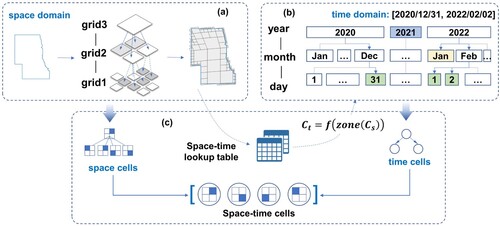
Figure 4. (a) Map and reduce phases of the aggregation query. (b) Spatial relationships between the cell and query domains.

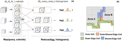
Figure 5. Implementation architecture of the histogram cube.

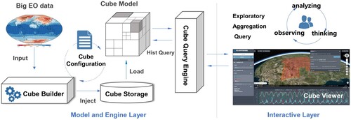
Figure 6. Implementation of the cube model layer. (a) Cube object. (b) Cube configuration. (c) Cube data storage.

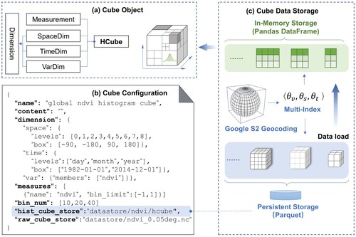
Figure 7. Workflow of the cube analysis process in the case study.

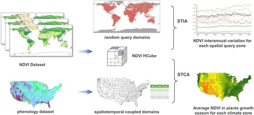
Figure 8. Cube building time and data reduction ratio in the case of different S2 cell sizes (a) and different numbers of histogram bins (b).

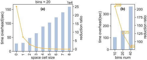
Figure 9. Response time of the individual aggregation queries with the increase in the space and time dimension on HCube-A. (a) ∼ (c) Performance of HCube and XCube with space growth. (d) ∼ (f) Performance of HCube and XCube with time growth (HCube and XCube). (g) ∼ (h) Performance of ArcGIS with space and time growth.

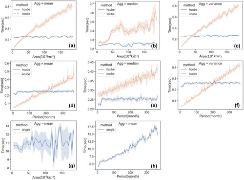
Figure 10. Response time of the individual aggregation queries along with space and time dimension growth on HCube-B. (a) ∼ (c) Performance with space growth. (d) ∼ (f) Performance with time growth.

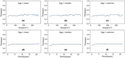
Figure 11. Performance of the concurrent STIA queries. (a) ∼ (f) show the resource overhead (Energy, CPU, Mem, Read and Write) and response time in the querying process. (g) ∼ (h) show the comparative curves of CPU and memory utilization in the aggregation process for the mean.

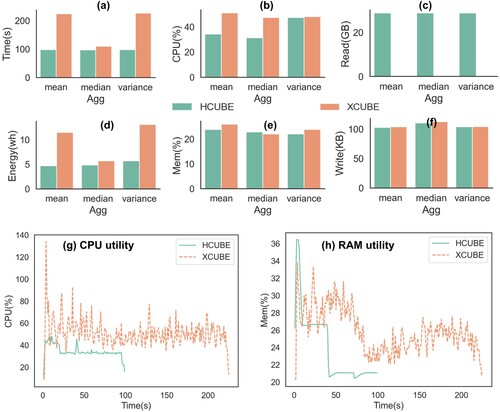
Figure 12. Variation in the response time along the space domain for the individual STIA query tasks in a concurrent environment, where (a) Agg = mean, (b) Agg = median, and (c) Agg = variance.

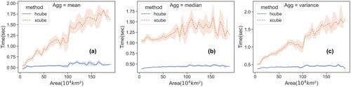
Figure 13. Performance comparison of STCA and STIA. (a) Response time. (b) Energy consumption. (c) CPU utilization. (d) Memory usage.

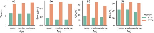
Figure 14. Errors of the aggregates (sum, mean, median, and variance) with space and time dimension change. (a) ∼ (d) show the error variations with space growth. (e) ∼ (h) show the error variations with time growth. Relative errors are used in the case of the sum and variance.

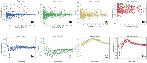
Figure 15. Error distribution of the aggregates (sum, mean, median, and variance) with histogram granularity (number of bins = [10, 20, 40]) and geographical latitude. Among the aggregates, rsum is the result of the sum after boundary correction. Note that the error value is the absolute value of the relative error.

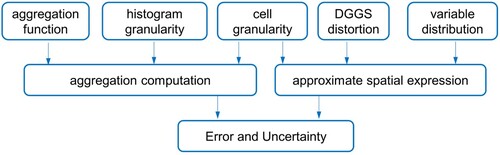
Figure 16. Factors influencing the query errors and uncertainties in HCube.

Data availability statement

The datasets of vegetation index and phenology for this study are openly available in https://vip.arizona.edu and http://www.nesdc.org.cn. The climate zone data for tests are available in National Center for Environment Information of US at https://www.ncei.noaa.gov. The additional materials that support the findings of this study are available on request.