Suitability analysis of human activities over Antarctic ice shelves: an integrated assessment of natural conditions based on machine learning algorithms

Figures & data

Figure 1. The location of ice shelves, stations, camps and field sites used in this study.

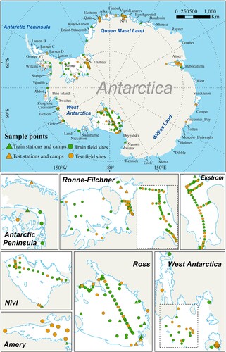
Figure 2. The indicators applied in the HAS map: (a) crevasses, (b) blue ice, (c) slope, (d) wind, (e) strain rate, (f) max buttressing, (g) snow accumulation, (h) ice velocity and (i) air temperature.

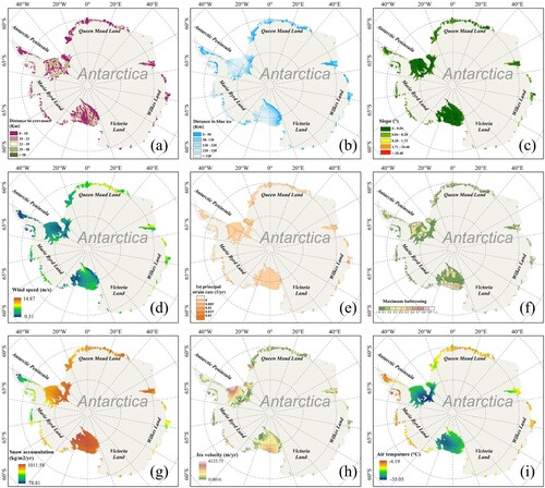
Table 1. Summary of the indicators used in our study.

Indicators	Source	Period	Spatial resolution	Correlation with HAS
Distance from Crevasses	Sentinel-1, MODIS	2021, 2009	500 m	Negative
Distance from blue ice area	MODIS	2014	500 m	Positive
Strain rate	MEaSUREs	2007–2018	450 m	Negative
Wind speed	ERA-5	2017–2021	0.10°	Negative
Snow accumulation	BAS	2001	1 km	Negative
Slope	ICESat-2	2020	500 m	Negative
Maximum buttressing	MODIS	2003	125 km	Positive
Air temperature	ERA-5	2017–2021	0.10°	Negative
Ice velocity	MEaSUREs	2007–2018	450 m	Negative

Figure 3. The methodological flowchart.

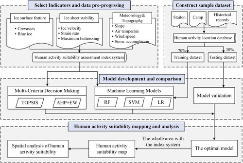
Figure 4. Factor importance estimates obtained by the developed RF model.

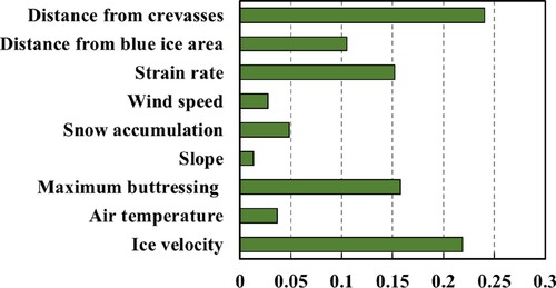
Table 2. Tolerance and VIF values in multicollinearity diagnosis test for the selected indicators.

Indicator layer	Tolerance	VIF
Distance from Crevasses	0.79	1.26
Distance from blue ice area	0.65	1.54
Strain rate	0.88	1.14
Wind	0.72	1.38
Snow accumulation	0.49	2.05
Slope	0.88	1.13
Maximum buttressing	0.69	1.45
Air temperature	0.38	2.61
Ice velocity	0.58	1.72

Figure 5. The five developed models’ ROC curves with training dataset (a) and testing dataset (b).

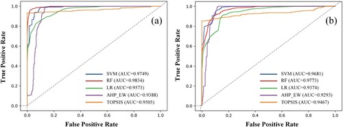
Table 3. Three statistical metrics of the machine learning model.

Statistical metrics	Training dataset			Testing dataset
	SVM	RF	LR	SVM	RF	LR
Overall accuracy	0.9516	0.9780	0.9438	0.9458	0.9639	0.9363
Kappa index	0.9032	0.9560	0.8877	0.8916	0.9479	0.8726
RMSE	0.1627	0.1520	0.1806	0.1739	0.1612	0.1889

Figure 6. The final HAS map by RF model. We divide Antarctica ice shelves into seven regions, which are labeled and delimited by line segments in dark blue. For each region, we compute area percentages of five HAS classes (pie charts). Yellow represents the testing dataset, green represents the training dataset. Triangle represents the research station sites, and circle represents the human activity records.

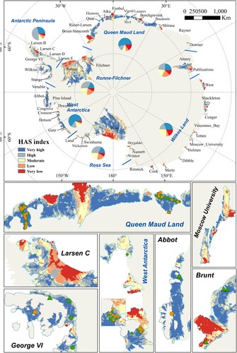
Table 4. Mean values of the selected indicators for the five HAS classes.

Parameter	HAS classes
	Very high	High	Moderate	Low	Very low
HAS index	1 - 0.83	0.83 - 0.63	0.63 - 0.43	0.43 - 0.22	0.22 - 0
Distance to crevasses (Km)	16361.09	15069.99	12724.17	10104.06	3446.96
Distance to blue ice (Km)	135674.68	146677.67	198421.92	206022.09	177121.63
Slope (°)	0.09	0.10	0.16	0.32	0.37
Wind speed (m/s)	3.23	3.18	3.21	3.99	3.76
Strain rate (1/yr)	0.0030	0.0052	0.0065	0.0062	0.0066
Buttressing (dimensionless)	0.51	0.25	0.14	0.09	0.08
Snow accumulation (kg/m2/yr)	218.54	203.00	209.60	238.10	248.42
Ice velocity (m/yr)	129.45	261.35	523.23	686.87	857.57
Air temperature (°C)	−18.44	−20.34	−22.15	−22.45	−19.57

Figure 7. Proportion of area for each HAS class within different ice shelves.

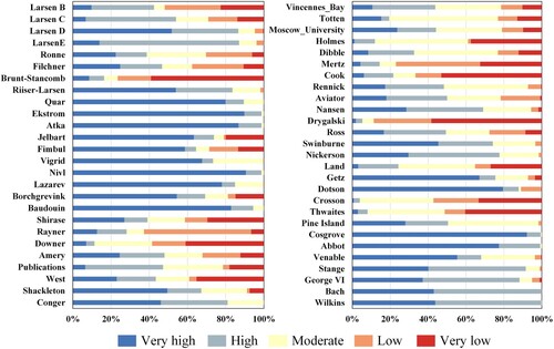
Figure 8. Crevasse and blue ice areas (a), HAS index (b), ice velocity (c), maximum buttressing (d) and strain rate (e) of the Ross ice shelf.

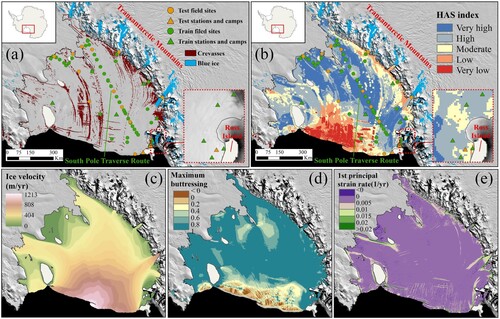
Figure 9. Crevasse and blue ice areas (a), HAS index (b), ice velocity (c), maximum buttressing (d) and strain rate (e) of the Ronne-Filchner ice shelf.

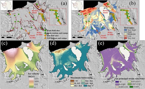
Figure 10. Crevasse and blue ice areas (a), HAS index (b), ice velocity (c), maximum buttressing (d) and strain rate (e) of the Amery ice shelf.

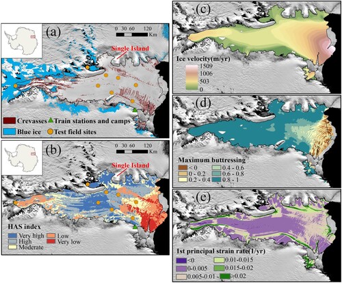
Figure 11. Comparison of results based on MCDA and machine learning models. (a) Generated HAS maps based on five models and the pairwise correlation coefficients for these maps, (b) Area and relative percentage for different HAS classes.

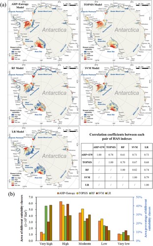
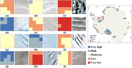
Figure 12. Characteristics of HAS index and Sentinel-2 data over Antarctic ice shelves. (a) Larsen C. (b) Larsen D. (c) Brunt. (d) Baudouin. (e) Shackleton. (f) Moscow University. (g, h) Nansen. (i) Getz. (j) Dotson. (k) Crosson. (l) Pine Island.

Data availability statement

Data are openly available in a public repository. Antarctic coastline and groundling data used in this study are from National Ice Center (https://usicecenter.gov/Resources/AntarcticShelf). The ERA5 reanalysis data were downloaded from the website (https://cds.climate.copernicus.eu/). The Antarctic ice velocity data were downloaded from the website (https://nsidc.org/data/nsidc-0484/versions/2). The MODIS Mosaic of Antarctica data were downloaded from the website (https://nsidc.org/data/nsidc-0730/versions/1). The fracture location map of Lai et al. (2020) is available at https://doi.org/10.15784/601335. The snow accumulation data were downloaded from the website (https://legacy.bas.ac.uk/bas_research/data/online_resources/snow_accumulation/index.php). The ICESat-2 DEM data were downloaded from the website (https://data.tpdc.ac.cn/en/disallow/9427069c-117e-4ff8-96e0-4b18eb7782cb/). Sentinel-1 imagery is available in Google Earth Engine (https://earthengine.google.com/).