
Figures & data
Figure 1. Four potential transformation patterns of urban spatial structures (adapted from Burger and Meijers (Citation2010)).
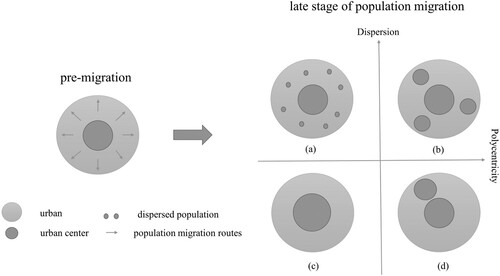
Figure 2. Cartographic representation of southeastern China. Blue regions represent the study area of this work.
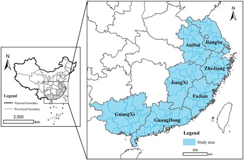
Figure 3. Spatial distribution of nighttime light intensity (a–f) in the southeastern region from 2012 to 2017.
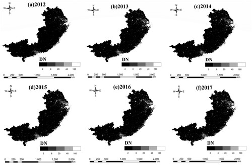
Figure 4. Framework of the methodology. GDP: gross domestic product per capita, NDVI: normalized difference vegetation index; TEC: number of patents, TNL: total nighttime light intensity, ICE: industrial carbon emissions, PCE: power carbon emissions, CCE: civilian carbon emissions, and TCE: transportation carbon emissions.
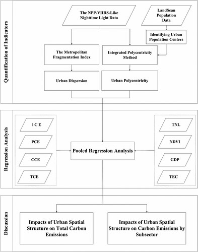
Figure 5. Box plots of urban dispersion and urban polycentricity from 2012 to 2017.
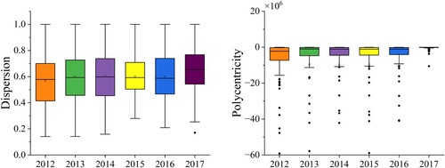
Figure 6. Spatial distribution of (a and b) urban dispersion and (c and d) polycentricity in 2012 and 2017. a(1), c(1), c(2), c(3), and c(4) represent Chizhou, Heyuan, Jieyang, Xiamen, and Suzhou, respectively.
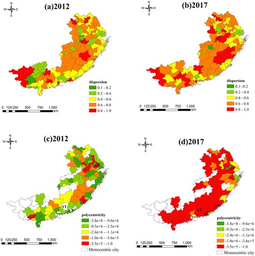
Table 1. Relations between urban spatial structures and carbon emissions.
Figure 7. Scatter plots of urban (a–f) dispersion and (g–l) polycentricity based on NTL data and traditional built-up area and urban center area from 2012 to 2017.
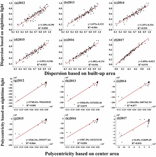
Table 2. Relations between urban spatial structures and carbon emissions in small and medium-sized cities.
Table 3. Relations between lag-phase urban spatial structure and carbon emissions.
Data availability statement
The NPP-VIIRS-like NTL data are freely available and downloadable from https://doi.org/10.7910/DVN/YGIVCD. Carbon emission data were derived from the Multi-resolution Emission Inventory for China (MEIC) model.