AttGAN: attention gated generative adversarial network for spatio-temporal super-resolution of ocean phenomena

Figures & data

Figure 1. The GAN architecture. The Attention 3D U-Net in the generator encodes the low-resolution input into an implicit feature grid. The ‘imnet’ decodes the implicit feature grid at each coordinate into the values of the original physical variables to construct the high-resolution predicted values. The predicted values are compared with the ground truth, and a regression loss is determined. Simultaneously, the predicted values are input into a discriminator to obtain an adversarial loss. Furthermore, the PDE loss is constructed by incorporating physical constraints represented by partial differential equations. This completes one cycle of adversarial training.

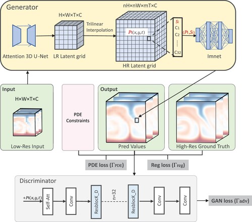
Figure 2. The generator structure. The generator integrates the attention gate modules and residual blocks and incorporates decoding networks related to physical constraints to enhance the reliability and accuracy of super-resolution predictions of the original physical quantities.

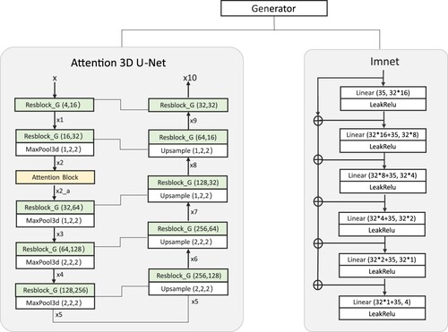
Table 1. The design details of the Attention 3D U-Net.

Input (C  ×  T  ×  H  ×  W)	Operator	Out_channel	Parameter
x0 (4  ×  4  ×  16  ×  16)	ResBlock_G	16	–
x1 (16  ×  4  ×  16  ×  16)	ResBlock_G + MaxPool3d	32	(1,2,2)
x2 (32  ×  4  ×  8  ×  8)	Attention gate module	32	–
x2_a (32  ×  4  ×  8  ×  8)	ResBlock_G + MaxPool3d	64	(1,2,2)
x3 (64  ×  4  ×  4  ×  4)	ResBlock_G + MaxPool3d	128	(2,2,2)
x4 (128  ×  2  ×  2  ×  2)	ResBlock_G + MaxPool3d	256	(2,2,2)
x5 (256  ×  1  ×  1  ×  1)	ResBlock_G + Upsample	128	(2,2,2)
x6 (128  ×  2  ×  2  ×  2)	cat (x6, x4)	256	–
x6' (256  ×  2  ×  2  ×  2)	Upsample + ResBlock_G	64	(2,2,2)
x7 (64  ×  4  ×  4  ×  4)	cat (x7, x3)	128	–
x7' (128  ×  4  ×  4  ×  4)	Upsample + ResBlock_G	32	(1,2,2)
x8 (32  ×  4  ×  8  ×  8)	cat (x8, x2)	64	–
x8' (64  ×  4  ×  8  ×  8)	Upsample + ResBlock_G	16	(1,2,2)
x9 (16  ×  4  ×  16  ×  16)	cat (x9, x1)	32	–
x9' (32  ×  4  ×  16  ×  16)	ResBlock_G	32	–
x10 (32  ×  4  ×  16  ×  16)	output	32	–

Figure 3. Basic blocks in the generator and discriminator.

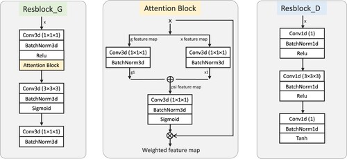
Figure 4. The discriminator network architecture.

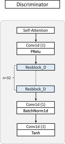
Figure 5. The visualization of salinity at t = 167 T of the ISWs in the South China Sea predicted by AttGAN. Each grid on the axis represents 71 km. The red dashed box in (c) indicates the more prominent waveform features of the ISWs. (a) Ground Truth. (b) Low-resolution input and (c) AttGAN (ours).

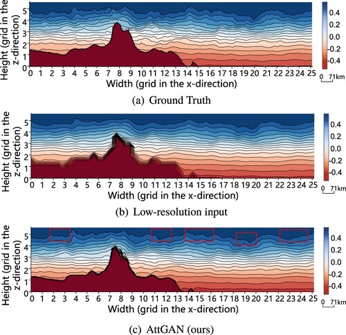
Figure 6. The visualization results of temperature at any point in time in the observation of the ISWs predicted by the proposed AttGAN model. The red dashed box in (c) indicates the more prominent waveform features of the ISWs, which are missing from the low-resolution input. (a) Low-resolution input of temperature channel. (b) Ground Truth and (c) AttGAN (ours).

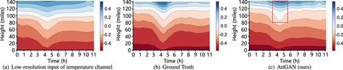
Figure 7. Low-resolution input of temperature channel. Each grid on the axis represents 4 m.

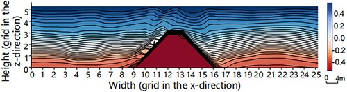
Table 2. Quantitative comparisons of different methods on ISWs.

Figure 8. Visual comparisons of different methods for the temperature at t = 82 T, including the ground truth, the proposed model's result, the MeshFreeFlowNet model's result, and the TransFlowNet model's result. Each grid on the axis represents 3 km. The red dashed box reveals differences in the restored waveform features between the three models. The proposed model's result was the closest to the ground truth, followed by the MeshFreeFlowNet model. (a) Ground Truth. (b) AttGAN (ours). (c) MessFreeFlowNet and (d) TransFlowNet.

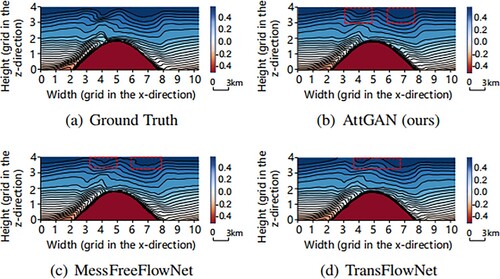
Figure 9. Low-resolution input of temperature channel. Each grid on the axis represents 80 m.

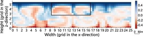
Figure 10. Visual comparison results of different methods for the temperature component at $t=92$ T. Each grid on the axis represents 6 m. Compared to the ground truth, the result of the MessFreeFlowNet exhibited noticeable biases (particularly in the lower center of the vortex on the left). The TransFlowNet introduced some grid-like artifacts, and the proposed AttGAN achieved the best result among all the models. (a) Ground Truth. (b) AttGAN (ours). (c) MessFreeFlowNet and (d) TransFlowNet.

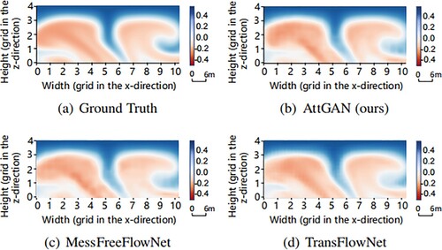
Table 3. Quantitative comparisons of different methods on Rayleigh–Bénard.

Table 4. Ablation study results of AttGAN using the ISWs dataset.

Design	S		T		u		w		Average
	PSNR	SSIM	PSNR	SSIM	PSNR	SSIM	PSNR	SSIM	PSNR	SSIM	Amp MSE
AttGAN (alpha = 0.0125)	33.9192	0.9926	39.6518	0.9936	43.6542	0.9879	44.9015	0.9897	40.5317	0.9909	0.0889
No_attBlock	33.1368	0.9915	38.4394	0.9924	44.1019	0.9883	44.3956	0.9890	40.0184	0.9903	0.0843
No_G_resblock	32.5625	0.9908	37.8966	0.8740	42.2621	0.9747	42.2488	0.9997	38.7425	0.9598	0.1833
No_D_resblock	32.3296	0.9920	39.8961	0.9935	43.4066	0.9879	44.8158	0.9893	40.1120	0.9907	0.1181
pde_alpha = 0.0	32.4331	0.9916	39.1179	0.9930	44.0051	0.9881	44.5461	0.9892	40.0256	0.9905	0.0955
pde_alpha=0.01	32.6950	0.9919	38.9379	0.9927	43.2541	0.9869	44.2651	0.9886	39.7880	0.9900	0.1340
pde_alpha=0.03	33.0056	0.9917	38.2447	0.9918	42.9394	0.9868	44.5880	0.9890	39.6945	0.9898	0.1592
pde_alpha=0.05	33.3694	0.9924	37.6176	0.9897	43.0222	0.9876	44.6612	0.9893	39.6676	0.9897	0.1026
pde_alpha=0.07	34.0656	0.9928	35.8669	0.9853	42.7689	0.9857	44.4598	0.9891	39.2903	0.9882	0.1443

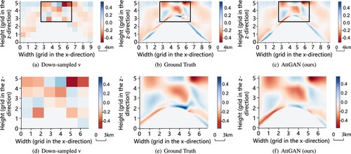
Figure 11. Visualization results of slices of velocity component v ($\times 16$) at t = 41 T predicted by the proposed AttGAN. In (a)–(c), each grid on the axis represents 4 km; in (d)–(f), each grid on the axis represents 3 km. The result predicted by the proposed model was close to the ground truth. (a) Down-sampled v. (b) Ground Truth. (c) AttGAN (ours). (d) Down-sampled v. (e) Ground Truth and (f) AttGAN (ours).

Data availability statement

The data that support the findings of this study are openly available in Zenodo at https://doi.org/10.5281/zenodo.10472771

 Google Scholar

.