Predicting time series of vegetation leaf area index across North America based on climate variables for land surface modeling using attention-enhanced LSTM

Figures & data

Figure 1. The map of vegetation types across the continent of North America. The red points indicate the locations of flux tower sites.

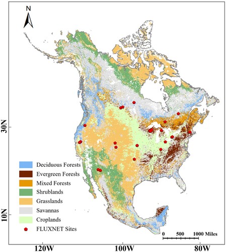
Figure 2. AELSTM model architecture. The attention enhanced layer is indicated by the red line. The red dashed boxes in the LSTM network den ote the memory flow of the forget gate, input gate, and output gate. In the feature matrix, T denotes the length of the time sequence, n denotes the input time steps, a-g represent the meteorological variables.

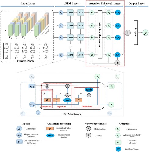
Figure 3. The spatial distributions AELSTM LAI, MODIS LAI, and MAE on four typical days in 2016: May 5 in spring, August 1 in summer, November 5 in autumn, and February 6 in winter. The fourth column shows the latitudinal profiles of the above LAI results where the shading denotes the standard deviation.

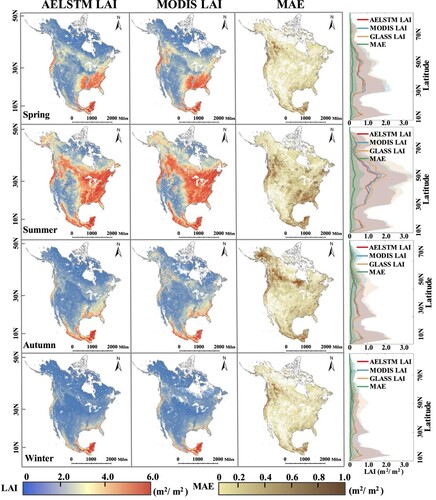
Figure 4. Comparison of AELSTM LAI and MODIS LAI under different biome types. P is the percentage of image elements with uncertainty within 20%. The blue dashed line is the fit line.

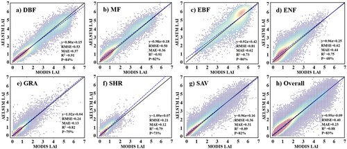
Figure 5. Comparison of AELSTM LAI, MODIS LAI, GLASS LAI, and FLUXNET LAI at ground sites across various biome types from 2009 to 2016. The name and coordinates of each FLUXNET site are indicated in the upper left corner of the subplot. The R² values marked with black, blue, and orange indicate the correlation coefficient between the AELSTM LAI and the MODIS LAI GLASS LAI, FLUXNET LAI, respectively.

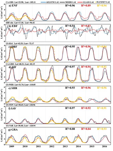
Figure 6. The approximate ranges of AELSTM LAI and MODIS LAI for different biome types.

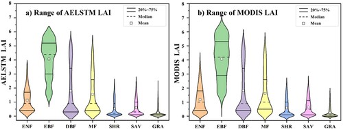
Figure 7. The 8-year averaged MAE and R² (indicated by different colors) between AELSTM LAI and MODIS LAI from 2009 to 2016 for different biome types over the day of year.

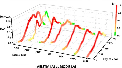
Table 1. Model evaluation of the machine learning and deep learning models.

Models		DV			EV			SDV
	R^2	RMSE m^2/m^2	MAE m^2/m^2	R^2	RMSE m^2/m^2	MAE m^2/m^2	R^2	RMSE m^2/m^2	MAE m^2/m^2
AELSTM	0.93	0.473	0.314	0.90	0.498	0.288	0.92	0.202	0.115
GRU	0.85	0.613	0.41	0.79	0.732	0.533	0.86	0.285	0.163
BiLSTM	0.86	0.682	0.421	0.83	0.597	0.426	0.83	0.353	0.189
RNN	0.79	0.860	0.482	0.82	0.634	0.418	0.84	0.336	0.176
LSTM	0.90	0.545	0.391	0.85	0.593	0.386	0.88	0.268	0.147
RF	0.87	0.578	0.436	0.83	0.638	0.436	0.86	0.335	0.207
CNN	0.81	0.71	0.523	0.81	0.662	0.424	0.83	0.351	0.236
SVM	0.84	0.637	0.457	0.76	0.684	0.581	0.85	0.318	0.186

Figure 8. AELSTM model validation at FLUXNET sites. The scatter density plots illustrate the comparisons between the satellite-derived LAI and AELSTM-predicted LAI for various vegetation types at the site scale.

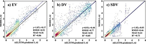
Figure 9. Comparison of the GPP results from the CoLM2014 using MODIS LAI and AELSTM LAI. Subplot (a) and (c) show the GPP predicted using the AELSTM LAI. Subplot (b) and (d) show the GPP predicted using the MODIS LAI. Subplot (e) and (f) present the latitudinal GPP averages, where the shading denotes the standard deviation. The scatter plots in subplot (a) and (c) show the regression analysis of predicted GPP using MODIS LAI and AELSTM LAI from CoLM.

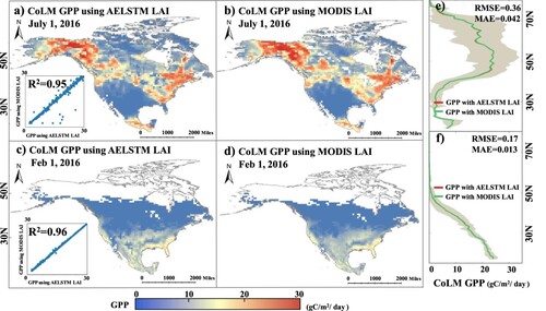
Figure 10. The spatial distribution of AELSTM LAI predicted under three shared socioeconomic pathways (SSPs), compared with that for CMIP6 LAI. Panel (a)–(d), (e)–(h), and (i)–(l) show the predicted LAI results under SSP 126, SSP 370, and SSP 585, respectively.

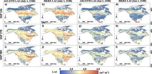
Figure 11. Time series of annual mean AELSTM LAI predicted under three SSPs from 2060 to 2100, compared with that for DKRZ LAI. The R² and MAE indicate the AELSTM performance under SSP126, SSP370, and SSP585, respectively.

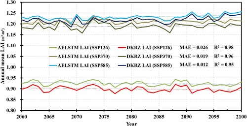
Figure 12. Comparison of the predicted LAI results using different modeling methods in summer and winter. The first column shows the AELSTM LAI obtained using the pixel-based method, the second column shows that obtained using the biome-based method, the third column shows the MODIS LAI for reference, and the fourth column shows the latitudinal profiles of the above LAI results where the shading denotes the standard deviation. The metrics (R², BIAS, RMSE) in subplot (a), (b) and (d), (e) are calculated with MODIS LAI.

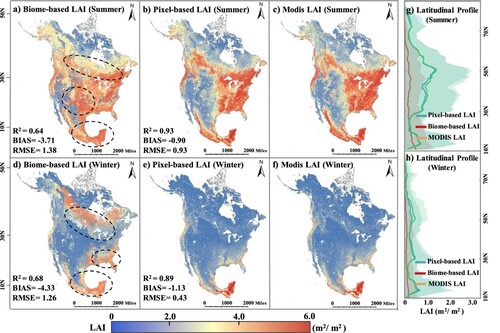
Table 2. Variations in model performance after a specific meteorological variable is omitted.

	Day length	Maximum temperatures	Minimum temperatures	Vapor pressure	Shortwave radiation	Snow water equivalent	Precipitation
RMSE	0.84	0.14	0.13	0.10	0.09	0.08	0.04
MAE	0.63	0.12	0.11	0.08	0.08	0.06	0.02
R^2	-0.10	-0.04	-0.03	-0.02	-0.02	-0.02	-0.01

Data availability statement

The authors thank Dai et al for providing the common land model (CoLM) Version 2014 code through the site: http://globalchange.bnu.edu.cn/research. The MODIS data sets including MOD15A2H, MCD12Q1, and MOD17 are available from https://ladsweb.modaps.eosdis.nasa.gov/search/order. The GLASS LAI product (version 6.0) is available for download from http://www.glass.umd.edu/Download.html. The FLUXNET 2015 is available at https://fluxnet.org/data/fluxnet2015-dataset. The Daymet dataset was downloaded from the Oak Ridge National Laboratory at http://daymet.ornl.gov/. We downloaded daily future climatic variables from the German Climate Computation Center (DKRZ) in Climate Model Intercomparison Project 6 (CMIP6) at https://esgf-node.ipsl.upmc.fr/search/cmip6-ipsl/. The AELSTM model package we proposed and code for analyses are available on the authors’ personal zenodo at https://zenodo.org/records/10395982. We welcome researchers and academics to further evaluate and improve the proposed model.

Acknowledgments

The authors thank anonymous reviewers for their constructive comments.