Modeling the spatial distribution of Spartina alterniflora ecological response to the interaction of flooding and soil salinity base on UAV data in Coastal Wetland

Figures & data

Figure 1. The location of the Dafeng Milu National Nature Reserve in Jiangsu Province. The background image is a natural true color drone photo taken on August 13, 2020. The unmanned aerial vehicle (UAV) provides a view of the field sample locations, showcasing the varying canopy heights and aboveground biomasses of S. alterniflora. The corresponding field photos, labeled as A, B, and C, were captured at these three sample locations in August 2020.

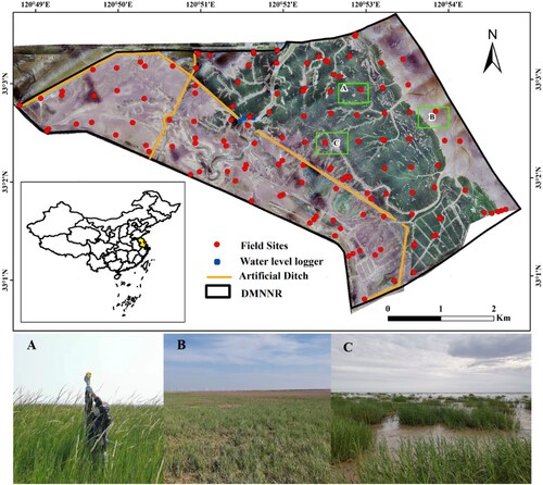
Figure 2. Two key components: (a) The digital elevation model (DEM) over the Dafeng Milu National Nature Reserve, and (b) The canopy height model (CHM) of S. alterniflora.

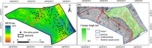
Figure 3. The flow chart of modeling the spatial distribution of S. alterniflora ecological response to the interaction of submergence and soil salinity (blue: data acquisition; green: method; Orange: result).

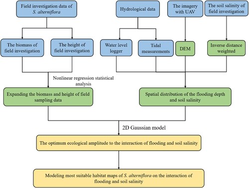
Figure 4. (a) The red solid line represents the daily average water level curve of the lunar calendar; (b) Spatial distributions of inundation depth, derived from the one-year water level curve and DEM, and (c) The spatial distribution of soil salinity across the Dafeng Milu National Nature Reserve.

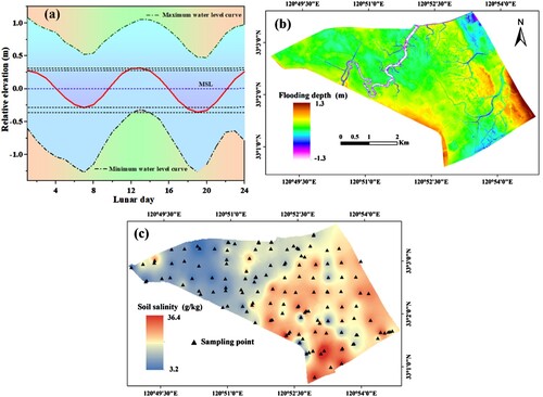
Figure 5. Spatial distribution of field verification points for S. alterniflora height and biomass.

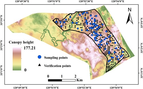
Table 1. The coefficients of the two-dimensional Gaussian regression model corresponding to S. alterniflora and the optimal ecological range of environmental factors.

Physiological Characteristics of S. alterniflora	Coefficient							Ecological Amplitude (u ± t) (P < 0.001)
	Z0	A	X0	Y0	W1	W2	R^2	Flooding depth	Soil salinity
Canopy height	43.12	134.09	0.39	17.83	0.69	8.96	0.73	0.39 ± 0.69 m	17.83 ± 8.96 g/kg
Aboveground biomass	657.36	2088.02	0.38	17.80	0.64	8.33	0.72	0.38 ± 0.64 m	17.80 ± 8.3 g/kg
Intersection of the optimal ecological amplitude								[0, 1.02 m]	[9.47, 26.13 g/kg]

Figure 6. The height (a) and aboveground biomass (b) of S. alterniflora along the interaction of inundation and soil salinity.

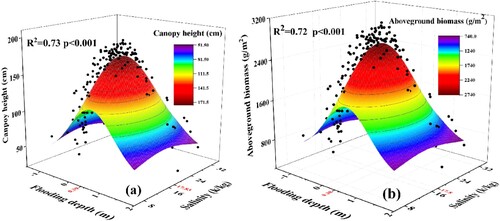
Figure 7. Spatial distribution map of the optimal habitat based on S. alterniflora canopy height for flooding depth(a), soil salinity (b), and canopy height (c).

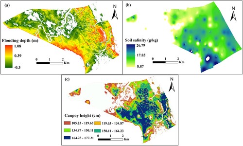
Figure 8. Spatial distribution map of the optimal habitat based on the S. alterniflora biomass for inundation depth(a); soil salinity (b) and aboveground biomass (c).

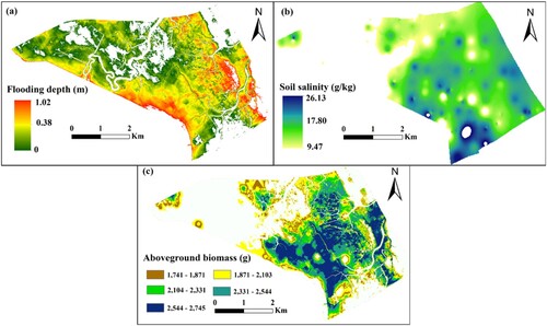
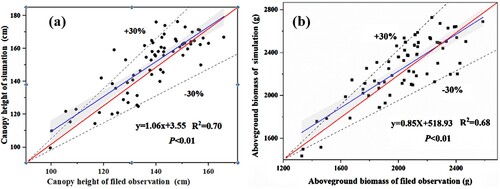
Figure 9. Scatter plots depicting the observed and simulated S. alterniflora height (a) and aboveground biomass (b). The blue solid line is Linear regression curve of measured values and simulated value of the S. alterniflora; The red solid line is standard line (y = x); the black dashed line is ± 30% error range.

Data availability

Data will be made available on request.