Contributions of Quaternary botany to modern ecology and biogeography

Figures & data

Table 1. Selected reviews on Quaternary floristic and vegetational history of different geographical areas. See Birks HJB and Berglund (2018) for further examples.

Region	References
Global	Huntley and Webb (1988); Tallis (1991)
Equatorial	Flenley (1979); Bush et al. (2011)
Canada	Ritchie (1984, 2008)
Eastern North America	Webb T et al. (1983a); Davis MB (1983b); Webb T (1988a); Grimm EC and Jacobson (2004)
South America	Urrego et al. (2009)
Europe	Huntley (1988)
Central Europe	Firbas (1949); Lang (1992, 1994)
Czech Republic	Kuneš and Abraham (2017)
Denmark	Iversen (1967, 1973)
Britain and Ireland	Godwin (1975)
Scotland	Edwards KJ et al. (2018)

Table 2. Selected reviews of contributions of Quaternary botany to modern ecology or biogeography.

General – dynamics, no-analogue assemblages, drivers of change, etc.	West RG (1964); Walker (1982a, 1990); Birks HJB (1986, 1993a); Bennett (1988b); Davis MB (1989c); Foster et al. (1990); Delcourt HR and Delcourt (1991); Ritchie (1991, 1995); Schoonmaker and Foster (1991); Huntley (1996); Mitchell FJG (2011); Luouys et al. (2012); Reitalu et al. (2014); Jackson and Blois (2015); Nogués-Bravo et al. (2018)
Resilience, diversity and stability	Walker (1982b, 1989)
Equilibrium–disequilibrium concepts	Davis MB (1986a)
Vegetation dynamics	Walker and Chen (1987); Prentice (1988a)
Interface between Quaternary botany and evolution	Bennett (1997)

Figure 1. (a) Mid-elevation belt of Pinus contorta, P. ponderosa, Picea engelmannii, Betula papyrifera, and Populus tremuloides between lowland xeric Artemisia tridentata sagebrush-steppe and high-elevation snow and dry open alpine vegetation, Borah Peak, Idaho, USA. This is a possible modern analogue for a'classical' macrorefugium for trees in the mountains of southern Europe during the last glacial maximum (LGM). Photograph: HJB Birks. (b) Local stands of Picea crassifolia along water seepages at 3600 m on the south-eastern Tibetan Plateau, Sichuan, China. This is a possible modern analogue for a 'microrefugium' for trees in Europe during the LGM. Modern pollen percentages of Picea at this site are less than 3%. Photograph: HJB Birks.

Figure 2. The glacial–interglacial cycle for north-west Europe showing the broad changes in biomass (above-ground productivity), soil status, and temperature that take place during a glacial stage (cryocratic – blue) and its associated interglacial stage (protocratic, mesocratic, oligocratic and telocratic – orange). The largest changes in temperature occur at the glacial–interglacial transitions; that is at the beginning and end of the cryocratic phase, particularly at the cryocratic–protocratic transition. There are also fine-scale climatic changes within an interglacial stage and a glacial stage. Based on Iversen (1958), Andersen ST (1994), and Birks HJB and Birks (2004). In the Holocene (present interglacial), the Homo sapiens phase (Birks HJB 1986) replaces the oligocratic and telocratic phases at sites with fertile soils (Birks HJB 1986).

Figure 3. Summary pollen diagram of the composite long pollen sequence from the Velay Plateau in the south-eastern part of the French Massif Central. The interglacial stages are shaded in pale brown and the corresponding marine isotope stages (MIS) are shown. Note the change between interglacial stages with dominant temperate trees and cold, dry glacial stages with dominant Poaceae and steppe taxa. The Holocene is MIS 1, the Ribains interglacial is MIS 5e (= Eemian), the Bouchet I interglacial is MIS 7c, the Landos interglacial is MIS 9e, and the Praclaux interglacial is MIS 11e (= Holsteinian). Redrawn and modified from de Beaulieu et al. (2001).

Figure 4. Comparison of interglacial tree pollen stratigraphies in five interglacial stages in the composite long pollen sequence from the Velay Plateau in the south-eastern part of the French Massif Central (Figure 3). Major tree pollen taxa are coloured identically between interglacials. The approximate age of the onset of each interglacial is also shown along with the correlations with marine isotope stages (MIS). Redrawn and modified from de Beaulieu et al. (2006).

Figure 5. Schematic diagram summarising the main stages and associated pedological changes (1–4) occurring in the transition from a podsol supporting coniferous forest in the late-glacial (stages 1 and 2) to a brown-earth soil with deciduous forest in the early-mid Holocene (stage 4) at Kis-Mohos Tó (NE Hungary) via an intermediate phase of a podsolic brown-earth with deciduous trees in the early Holocene (stage 3). The chemical record in the lake sediment at Kis-Mohos Tó is summarised. Redrawn from Willis et al. (1997).

Figure 6. Gerzensee, a kettle-hole lake on the Swiss Plateau at 603 m elevation (46.83°N, 7.55°E). This site has been the focus of detailed studies on rapid warming and associated biotic changes in the late-glacial and early Holocene (Ammann and Oldfield 2000; Ammann et al. 2013a, 2013b, 2013c), for example the study summarised in Figure 7. The Bernese Alps are in the background. Photograph: AF Lotter.

Figure 7. Vegetation and soil development around Termination A (Oldest Dryas/Bølling transition) about 14,665 calibrated years ago at Gerzensee, Switzerland (see Figure 6). Changes in stable oxygen-isotope ratios (δ¹⁸O‰) of bulk carbonate in the lake sediments (A) provide a climate proxy independent of the pollen stratigraphy. The physiognomy of the past vegetation (B) and vegetation type (C) are inferred from pollen (D) and plant-macrofossil data (the nitrogen-fixing shrub Hippophaë rhamnoides is shown in orange in B). Pollen-accumulation rates (grains cm^–2 yr^–1) (D) reflect vegetation cover and biomass, whereas rates of palynological change (per 70 yr) (E) highlight times of marked change shown by a small or big * that are 50% or 75% greater than the mean rate of change, respectively. Palynological richness (α-diversity) (F) is estimated as number of taxa cm^–2 yr^–1 to allow for the changes in pollen-accumulation rates (D). The inferred soils (G) are summarised in terms of the extent of the active layer, amount of nitrogen-fixation based on the abundance of nitrogen-fixing plants in the pollen and plant-macrofossil stratigraphies, and general soil types. Inferred changes in the potential nitrogen and phosphorus resources during the vegetation development are also shown (H). All the stratigraphical data are smoothed with a running mean over five samples. Redrawn and modified from Ammann et al. (2013b) and Birks HJB et al. (2016b).

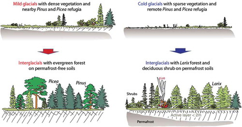
Table 3. Possible dominant mycorrhizal types and nitrogen fixers in a north-west European glacial–interglacial cycle and suggested levels of above-ground productivity, available soil phosphorus levels, and amount of nitrogen fixation. This scheme is based on many sources including Harley and Harley (1987), Read (1993a, 1993b), Cázares et al. (2005), Kuneš et al. (2011), and Dickie et al. (2013).

Stage Phase	Glacial Cryocratic	Protocratic	Interglacial Mesocratic	Oligocratic + Telocratic
Above-ground productivity	+	++	+++	++
Available P	+	+++	++	+
N fixation	+	+++	++	+
Vegetation	Herbs and open ground	Grassland, open scrub and woodland	Forest	Open forest, heaths, bogs
N-fixers	Dryas, legumes*	Dryas, legumes*	?
Mycorrhizal types
Arbuscular mycorrhiza	Salix, grasses	Juniperus, Salix, grasses	(P-scavengers) Ulmus, Fraxinus, Alnus, Taxus
Ectomycorrhiza	Dryas, Salix	Dryas, Betula, Salix, Populus	Quercus, Corylus	(P-miners) Pinus, Picea, Fagus
Ericoid mycorrhiza		Empetrum		Vaccinium, Empetrum
Non-mycorrhizal	Herbs	Herbs		Herbs

+ = low; ++ = medium; +++ = high

* Including Astragalus alpinus, Lotus corniculatus, Anthyllis vulneraria, Hedysarum spp., Oxytropis spp., and Trifolium spp., which have been found in cryocratic and protocratic pollen assemblages (e.g. Iversen 1954; Andersen ST 1961; Birks HJB 1973)

Figure 8. The series of pollen diagrams presented by Lennart von Post in his 1916 lecture in Kristiania along a south-west to north-east transect from Zealand (site F), through Skåne and Småland (sites 1–8) and into Västergötland, Östergötland, and Närke on the borders of the north and central Swedish uplands (sites 9–12). The southern limit of Picea abies lies between sites 3 and 4, and the northern limit of Fagus sylvatica is near site 6. The EK-Blandskog + Corylus curve is the combined values of Quercus, Ulmus, Tilia, and Corylus (‘Quercetum Mixtum’). The colours are those that von Post used in his original lecture-chart. As on all his diagrams, von Post has signed it in the bottom right-hand corner. Based on a diagram in Fries M (1967) but extensively modified. This series of pollen diagrams was subsequently published in very different formats by von Post (1924, 1926a).

Figure 9. Picea pollen percentages (expressed as percentages of total tree pollen) at over 250 sites in southern Sweden in the (1) Sub-Boreal, (2) early Sub-Atlantic, (3) middle Sub-Atlantic, and (4) recent times. The native southern range limit (in 1924) is indicated as a solid line on the map for recent times (4). Modified from von Post (1924).

Figure 10. Maps of Quercus (deciduous) pollen percentages across Europe for 12,000, 10,000, 8000, 6000, 4000, and 2000 radiocarbon years before present (BP) drawn as isopollen contours representing different percentage values (modified from Huntley and Birks 1983), and for 14,000, 11,500, 9000, 7000, 4500, and 2000 calibrated years BP drawn as different sized solid circles representing different pollen percentage values (modified from Brewer et al. 2017). The blue shading on the dot maps for 14,000 and 11,500 yr BP shows the likely extent of glacial ice in Fennoscandia. The two sets of maps have been approximately correlated in time using the IntCal13 radiocarbon calibration curve and CalPal (www.calpal-online.de) as the isopollen maps are in radiocarbon years BP and the dot maps are in calibrated years BP.

Table 4. Selected examples of Holocene isochrone maps for different geographical areas.

Area	References
Eastern North America	Moran (1973); Davis MB (1976, 1978, 1983a, 1983b, 1986a); Bernabo and Webb (1977); Jacobson GL (1979); Webb T (1981); Webb T et al. (1983a, 1983b); Björck (1985); Davis RB and Jacobson (1985); Gaudreau and Webb (1985); Davis MB et al. (1986)
Britain and Ireland	Birks HJB (1989)
Fennoscandia	Donner (1963); Aario (1965); Aartolahti (1966, 1967); Moe (1970); Persson (1975); Tolonen and Ruuhijärvi (1976); Høeg (1978); Tolonen (1983)
Russia	Serebryanny (1971, 1973)

Figure 11. Isochrones (in radiocarbon years BP) for Quercus pollen in Britain and Ireland. Modified from Birks HJB (1989).

Table 5. Estimated rates of spread (m yr^–1) of trees during the Holocene in Britain and Ireland (Birks 1989) and on the European mainland based on Huntley and Birks (1983), Feurdean et al. (2013), Brewer et al. (2017), and Giesecke and Brewer (2018).2017

	Britain and Ireland (Birks 1989)	Europe (Huntley and Birks 1983)	Europe – S (Feurdean et al. 2013)	Europe – N (Feurdean et al. 2013)	Europe (Brewer et al. 2017)	Europe (Giesecke and Brewer 2018)
Abies	-	40–300	205	170	200	250
Alnus	500–600	50–2000	225	100	200–500	600
Betula	250	>2000	540	260	?	800
Carpinus	-	50–1000	115	60	400	500
Corylus	500	1500	na	na	1000	1000
Fagus	100–200	200–300	130	90	300	400
Fraxinus	50–200	200–500	na	na	200	-
Picea	-	80–500	385	70	250	500
Pinus	<100–700	1500	360	195	?	600
Quercus	50–500	150–500	220	165	500	500
Tilia	50–500	300–500	na	na	500	500
Ulmus	100–550	500–1000	na	na	1000	1000

S = assuming spreading from southern macrorefugia only; N = spreading from northern microrefugia; ? = not estimable; na = not available

Figure 12. Possible scenarios for tree spreading across a large area in an interglacial stage. 1. The moving-front or continuous wave hypothesis where trees 'march' across the landscape. 2. Rare far-distance dispersal events form small outlying populations. 3. Populations expand from the outlying populations into locally favourable sites or enclaves. 4. Merging of large and small populations. Small scattered populations expand (as in 3) and are a source for dispersal events, as are the large populations. Scenarios 2, 3, and 4 combined are likely to be most important. Based, in part, on Davis MB (1987) and Giesecke (2013).

Table 6. Selected examples of range expansions or contractions of taxa that appear to show a ‘stop’ or ‘go’ behaviour during the Holocene.

Taxon/Taxa	Area	Reference
Abies alba and Fagus sylvatica	Central Europe	Tinner and Lotter (2006)
Betula alleghaniensis	Great Lakes region	Jackson and Booth (2002)
Conifers (mixed)	Yellowstone	Krause and Whitlock (2017)
Fagus grandifolia, Tsuga canadensis, and other trees	NE USA and Great Lakes region	Davis MB (1987); Woods and Davis (1989); Parshall (2002); Booth et al. (2004); Minckley et al. (2011); Clifford and Booth (2015)
Juniperus osteosperma	Rockies	Lyford et al. (2003)
Larix laricina	NW Quebec	Peñalba and Payette (1997)
Pinus contorta var. latifolia	Yukon	Edwards ME et al. (2015)
Pinus edulis	Utah	Gray et al. (2006)
Tsuga mertensiana	South-central Alaska	Anderson RS et al. (2017)

Figure 13. The changing relative abundance expressed as a percentage of the maximum attained values of tree taxa through time in Britain and Ireland. The top panel (1) shows how relative abundance changes through time in the absence of any detectable dispersal limitation or expansion limitation, as shown by the Holocene behaviour of Corylus, Populus, Salix, or Ulmus. The middle panel (2) shows relative abundance changes for taxa that experience dispersal limitation but little or no expansion limitation (e.g. Betula, Pinus). The bottom panel (3) shows relative abundance changes for taxa that may experience not only dispersal limitation but also prolonged expansion limitation (e.g. Alnus, Carpinus, Fagus) that may extend for 2000–3000 years. Of these, Alnus is the most extreme in its expansion limitation due to the rarity of its 'island-like' wet habitats. There are not enough detailed data to assess the long-term behaviour of Fraxinus, Quercus, or Tilia.

DL = Dispersal limitation; EL = Expansion limitation; EP = Expansion phase.

Figure 14. Suggested location of refugial areas for Fagus sylvatica during the last glacial maximum (blue circles) and the major spread into Europe during the Holocene (blue arrows). The green shaded areas are the present native range of F. sylvatica. Modified from Magri et al. (2006).

Table 7. Numbers of total and species partial extinctions and exterminations of taxa in recently studied Late Pliocene sequences in Belarus and Early or Middle Pleistocene interglacials in Poland along with their assumed correlations with Marine Isotope Stages (MIS) and interglacial stages in western Europe (Lindner et al. 2013). (Based on Stachowicz-Rybka 2015a and data from Mamakowa and Velichkevich 1993a; Velichkevich and Granoszewski 1996; Velichkevich and Lesiak 1996; Velichkevich and Mamakowa 2003; Velichkevich and Zastawniak 2003; Velichkevich et al. 2004; Stachowicz-Rybka 2011, 2015a, 2015b, 2015c; Drzymulska 2018).

	Estimated age (kyr)	MIS	Western Europe stage	Polish stage	Total extinctions	Species extinctions	Exterminations	Number of taxa identified
Middle Pleistocene	370–425	11	Holsteinian	Mazovian	1	5	4	198
	480–620	13–15	Cromerian IV	Ferdynandovian 2	0	17	4	174
Early Pleistocene	710–760	17	Cromerian III	Domuratovian and Ferdynandovian I (Podlasian p.p.)	0	12	3	155
	790–815	19/20	Cromerian II/Glacial A1	Augustovian (Podlasian p.p.)	0	13	3	147
	865–1000	21	Cromerian I	Podlasian p.p.	0	18	4	162
Late Pliocene				Kholmech	1	78	24	170

p.p. = in part

Table 8. Comparison of modern climatic requirements of cool-temperate tree genera that grew in Europe in the Neogene but had been exterminated by the early Pliocene, that were present in Europe in the Neogene but have relictual disjunct distributions today, and that were present in the Neogene and are widespread in Europe today (based on Svenning 2003). Minimum growing degree days and the moisture index (actual evapotranspiration/potential evapotranspiration) are only available for genera in North America.

	Regionally extinct in Europe	Relictual in Europe	Widespread in Europe
Cool-temperate tree genera	38	9	26
Mean temperature of the coldest month (°C)	−7.98 ± 6.39	−12.0 ± 5.76	−23.4 ± 9.14
Mean annual temperature (°C)	6.26 ± 4.00	4.26 ± 2.88	−4.47 ± 2.28
Mean annual precipitation (mm yr^–1)	547 ± 322	273 ± 206	274 ± 215
Growing degree days (°C)	1.4 ± 0.64	1.3 ± 0.41	0.37 ± 0.45
Moisture index (AET/PET)	0.54 ± 0.26	0.29 ± 0.23	0.28 ± 0.22

Table 9. Selected genera or species other than trees that were exterminated from north-west Europe during the Neogene or Pleistocene. See Tralau (1959, 1963a), van der Hammen et al. (1971), Huckerby and Oldfield (1976), Watts (1988), Lang (1994), Mai (1995), Drzymulska (2018), and Góis-Marques et al. (2019) for details.

Shrubs	Ferns
Clethra	Osmunda cinnamonea
Coriaria	O. claytonia
Corylopsis	Wetland shrubs or herbs
Eleagnus	Chamaecyparis thyoides
Fothergilla	Decodon verticillatus
Parthenocissus	Dulichium arundinaceum
Rhus	Aquatic plants
Staphylea	Azolla filiculoides
Styrax	Brasenia schreberi
Vines	Euryale ferox
Epipremnum	Nymphoides aquatica
Schizandra	Proserpinaca cf. palustris

Table 10. Selected examples of publications on the role of persistence, evolutionary adaptation, and of phenotypic plasticity in influencing biodiversity patterns today and in the future.

Holt (1990)	Nicotra et al. (2010)	Merilä and Hendry (2014)
Davis MB and Shaw (2001)	Sussman (2010)	Etterson et al. (2016)
Etterson and Shaw (2001)	Dawson TP et al. (2011)	Graae et al. (2018)
Davis MB et al. (2005)	Hill JK et al. (2011)	Henn et al. (2018)
Jump and Peñuelas (2005)	Hoffmann and Sgrò (2011)	Lallensack (2018)
Parmesan (2006)	Shaw RG and Etterson (2012)	Nogués-Bravo et al. (2018)
Aitken et al. (2008)	Alberto et al. (2013)
de Witte and Stöcklin (2010)	Franks et al. (2014)

Figure 15. (1) Fundamental, potential, and realised niches of a species in response to two environmental variables. The realised niche is where populations of the species actually occur and is a subset of the potential niche constrained by biotic, abiotic, and other factors. The potential niche is where the fundamental niche intersects with the realised environmental space at a particular time. (2) A schematic representation of how changes in the realised environmental space between time 1 and time 2 can affect species co-occurrences. At time 1, the potential niches of species 1 and species 2 overlap and the species can potentially co-occur at sites within the intersection. At time 2, the potential niches of the two species do not overlap and hence they will not co-occur in the realised world. (3) The four modes of population response of five species (a-e) to environmental change. Species a mode 1: persistence. Species b modes 1 and 2: shift within local habitat conditions. Species c modes 1, 2, and 3: spread to distant newly-suitable sites and disappear from some former sites. Species d modes 1 and 4: widespread extirpation without colonisation of new areas, thereby changing from being a widespread species to a local or rare species. Species e is the inverse of species d where a formerly rare species colonises extensive new areas. Redrawn from Jackson and Overpeck (2000).

Table 11. The frequency of the four modes of response in species populations and species combinations (‘associations’) within Europe and North America during the late-Quaternary.

Mode	Population	Associations
1. Persistence	Rare	Rare
2. Local shifts	Occasional – frequent	Occasional
3. Spreading, colonisation, and expansion	Common	? Rare
4. Local or regional extermination	Frequent	Common

Table 12. Suggested drivers within the realised environment space (RES) resulting in no-analogue pollen assemblages and possible no-analogue vegetation types during different stages in the late-Quaternary in north-west Europe and eastern North America.

Stages	Potential drivers within RES	References
Interglacials	Climate and seasonality ?Herbivores ?Lags in spreading and population expansion	Watts (1988); Bartlein et al. (1998); Sandom et al. (2014b); Past Interglacials Working Group of PAGES (2016)
LGM	Climate ?Herbivores ?Soils Low CO2	Iversen (1967, 1973); Godwin (1975); Lang (1994); Jackson et al. (2000b); Jackson and Williams (2004)
Late-glacial	Climate, especially seasonality induced by insolation change Herbivores Fire Soils	Iversen (1954, 1967, 1973); Cushing (1963); Birks HH (2003); Jackson and Williams (2004); Gill et al. (2009, 2012); Jones RA et al. (2017)
Early Holocene	Climate, especially seasonality induced by insolation change Lags in spreading or population expansion	Webb T (1981, 1987); Prentice (1983); COHMAP Members (1988); Wright et al. (1993); Birks HJB (2008)

Figure 16. The three major hypotheses (H1–H3) and processes for changes in pollen-assemblage composition and abundance: environmental forcing (H1), biotic interactions (H2), and neutral processes (H3) that can cause ecological drift (Jackson and Blois 2015). These processes may interact in the real world. Exogenous environmental change (e.g. climate change) may be a major driver of assemblage properties both directly and indirectly by influencing interactions between taxa and initiating neutral processes. Climate varies continuously and may influence processes within all three hypotheses to modify assemblage properties (Jackson and Blois 2015). The three underlying hypotheses H1, H2, and H3 correspond to the hypotheses discussed in the text. Modified from Jackson and Blois (2015).

Table 13. Estimates of tree-population doubling times (t_d = log_n(2/r); rounded to nearest 5 years) derived from pollen-stratigraphical data (PAR) from North America (Tsukada and Sugita 1982; Tsukada 1982c, 1982d; Bennett 1986, 1988a; MacDonald and Cwynar 1991; MacDonald 1993a; Fuller 1998; Edwards ME et al. 2015), England (Bennett 1983, 1988b), Central Europe (Giesecke et al. 2007; Bradshaw RHW et al. 2010), Italy (Magri 1989), north-east Australia (Walker and Chen 1987; Chen 1988), and Japan (Tsukada 1981, 1982a, 1982b, 1982c; Tsukada and Sugita 1982; Kito and Takimoto 1999). Modified from MacDonald (1993a).

Region		Taxon	Doubling time (years)
North America		Abies	410
		Alnus rubra	110–180
		Fagus grandifolia	240–445
		Picea	35–180
		Pinus contorta ssp. contorta	110–175
		Pinus contorta ssp. latifolia	80–1100
		Pseudotsuga menziesii	50–365
		Tsuga mertensiana	30–460
		Tsuga plicata	225–240
England		Alnus glutinosa	175–270
		Betula	60
		Corylus avellana	45
		Pinus sylvestris	75
		Quercus	80–140
		Tilia cordata	100
		Ulmus	30–68
Central Europe		Fagus sylvatica	200–430
Italy		Abies	1120
		Carpinus	370–1360
		Corylus	440
		Fagus	370–810
		Juniperus	1175
		Olea	620
		Pinus	1130
		Quercus (deciduous)	665–1290
		Tilia	720
		Ulmus	665
		Zelkova	715
Australia	Gymnosperm canopy trees	Agathis	200
		Podocarpus	240–355
	Angiosperm canopy trees	Balnops	170
		Blepharocarya	150
		Cunoniaceae	65–120
		Elaeocarpus	105–165
		Eugia	185
		Rapanea	150
	Secondary trees	Macaranga/Mallotus	90–105
		Moraceae/Urticaceae	80–110
		Trema	80–110
Japan		Cryptomeria japonica	265–1085
		Fagus	125–435
		Pinus	55

Table 14. Estimates of tree-population halving times (t_h = log_e(2/r); rounded to nearest 5 years) derived from pollen-stratigraphical data (PAR) from North America (Tsukada and Sugita 1982), England (Peglar 1993a; Peglar and Birks 1993), and Japan (Tsukada 1983).

Region	Taxon	Halving time (years)
North America	Castanea dentata	5–15
	Tsuga canadensis	35
England	Ulmus	5
Japan	Picea	200–580

Table 15. Estimates of tree-population doubling times (t_d = log_e(2/r); rounded to nearest 5 years) derived from pollen-stratigraphical data (PAR) from two sites in southern Ontario after the marked decline of Tsuga canadensis pollen at about 5400 years ago (calculated from data in Fuller 1998).

Region	Taxon	Doubling time (years)
Ontario, Canada	Acer saccharum	350–695
	Betula	350–695
	Fagus gradifolia	230–695
	Pinus banksiana/resinosa	350–695
	Pinus strobus	695
	Quercus	350
	Thuja/Juniperus	230–695
	Tsugao canadensis	760–1000

Table 16. Estimates of tree-population doubling times (t_d = log_e(2/r); rounded to nearest 5 years) calculated from the eigenvalue (λ) of the transition matrix where log_eλ = r (see Piñero et al. 1984). Data from various sources compiled and documented by Bennett (1986).

Taxon	Doubling time (years)
Araucaria cunninghamii	35
Araucaria hunsteinii	10–15
Astrocaryon mexicanum	20
Nothofagus fusca	25
Pentaclethra macroloba	350
Podocarpus barteri	55
Sequoia sempervirens	165

Figure 17. Generalised pollen-stratigraphical patterns and inferred population processes suggested by Watts (1973) in the establishment and expansion of a tree in the mesocratic phase within an interglacial stage. The very approximate durations of the establishment and expansion intervals are also shown. Modified from Birks HJB and Tinner (2016a).

Figure 18. Hypothetical pollen-stratigraphical reflections of the same climate oscillation in different regions along an imaginary transect from south to north. In the far north, locality A, the climatic oscillation results in a retreat of tundra and expansion of ice. Locality B records the classical Allerød–Younger Dryas–early Holocene pattern of Betula woodland–tundra–Betula woodland. Farther south, the climatic oscillation is recorded by other vegetational and hence pollen-stratigraphical changes. Note that at localities D and F no major pollen-stratigraphical changes are observed as no ecotones are crossed. Based on Fægri and Iversen (1950).

Figure 19. Contrasts between an abrupt extrinsically forced ecological change (left panels) with an abrupt intrinsically forced change (right panels). In the extrinsically forced change, a large widespread change in temperature (a), e.g. the Younger Dryas–Holocene transition, causes abrupt ecological changes that are synchronous with or slightly lag behind the climate change at sites 1, 2, and 3 (c), resulting in a strong temporal coherence of change (e). With intrinsically forced change, a long-term progressive trend such as droughts and megadroughts (b) are mediated by site-specific (1–6) thresholds (d). These site-specific thresholds cause abrupt changes across the drought period (f). Clusters of site-level abrupt changes may result from extreme events which may impact many sites simultaneously (f). Modified from Williams et al. (2011a).

Figure 20. (a) The ecological thresholds for the establishment of prairie, oak (Quercus) woodland, and mixed deciduous forest (Bigwoods) in central Minnesota plotted along a climatic gradient (e.g. precipitation) that influences fire frequency. Redrawn from Grimm EC (1983). (b) Schematic representation of ecological thresholds for the establishment of prairie and woodland in central Minnesota. The horizontal axis is time; the vertical axis is a climatic gradient (e.g. mean annual precipitation). In the upper right quadrant (woodland only) above the woodland threshold for annual precipitation (Pw), only woodland will persist as a stable state once it is established. Either of two potentially stable states – woodland or prairie – can persist in areas with climate delimited by the thresholds for woodland (Pw) and prairie (Pp), while only prairie will persist as a stable state below the critical threshold for annual precipitation (Pp) and for increased fire recurrence (lower right quadrant: prairie only). Tw represents the minimum time required for woodland to invade prairie. The vegetation outcomes and pathways are summarised in the right-hand column. Redrawn from Grimm EC (1983) and Delcourt HR and Delcourt (1991).

Table 17. Selected examples of detailed fire histories reconstructed from charcoal in Quaternary botanical sequences with emphasis on interactions of fire with other variables, and rapid state shifts and system dynamics.

Interaction of fire, climate, vegetation, biomass and fuel-load, land use, and fauna	Rapid state shifts, alternative stable states, alternative transient states, abrupt changes (‘tipping points’) and system dynamics
Camill et al. (2003)	Walker (1982b)
Szeicz et al. (2003)	Tausch et al. (1993)
Craine and McLauchlan (2004)	Franklin SB and Tolonen (2000)
Umbanhowar (2004)	Lytle (2005)
Lynch et al. (2006, 2014)	Fukami and Nakajima (2011)
Umbanhowar et al. (2006)	Minckley et al. (2012)
Hotchkiss SC et al. (2007)	Fletcher et al. (2014b)
Shuman et al. (2009)	Calder and Shuman (2017, 2019)
Frégeau et al. (2015)	Crausbay et al. (2017)
Brussel et al. (2018)	Jeppesen et al. (2018)
Carter VA et al. (2018a)	Ratajczak et al. (2018)
Finsinger et al. (2018)	Stevens-Rumann et al. (2018)
Mariani et al. (2019)	Calder et al. (2019)

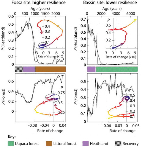
Table 18. Selected examples of recent theoretical and Quaternary studies on ecosystem dynamics, in particular regime shifts.

Theoretical studies
Scheffer et al. (2001, 2012, 2015) Andersen T et al. (2009) Contamin and Ellison (2009) Brock and Carpenter (2010)	Drake JM and Griffen (2010) Scheffer (2010) Carstensen and Weydmann (2012) Dakos et al. (2015)	Burthe et al. (2016) Ratajczak et al. (2018) Taranu et al. (2018)
Quaternary botanical studies on detecting regime shifts, thresholds, and tipping points
de Boer et al. (2013b) Davies (2016b)	Morris et al. (2019)	Stegner et al. (2019)
Palaeolimnological studies on detecting regime shifts, early-warning signals of a critical transition, thresholds, and tipping points
Randsalu-Wendrup et al. (2012, 2014, 2016) Wang R et al (2012) but see Carstensen et al. (2013)	Seddon et al. (2014b) Bunting L et al. (2016)	Ramstack Hobbs et al. (2016) Beck et al. (2018) Taranu et al. (2018)

Table 19. Approximate age of modern British woodland assemblages inferred from pollen-analytical stratigraphies and macrofossil data. The assemblages are based on the dominant tree taxa as indicated from pollen and/or plant macrofossil taxa. To aid vegetation reconstruction, fossil tree-pollen values have been transformed by Andersen’s (1970) general pollen representation factors as modified for British taxa (Edwards ME 1986). The antecedent pollen assemblage or vegetation type are based on available dated pollen data from Britain (Birks HJB 1989; Bennett and Birks 1990; Fyfe et al. 2010, 2013; Brewer et al. 2017). For details of the NVC types, see Rodwell et al. (1991).

Assemblage	NVC type	Estimated age of assembly (cal kyr BP)	Antecedent assemblage or vegetation type
Modern assemblages
Salix spp. woodland	W1 – 3	13.5	Late-glacial tall herb vegetation
Betula spp. woodland	W4	12.9	Juniperus and Salix scrub, herbs
Alnus glutinosa woodland	W5, W6	6.3–7.8	Salix woodland
Alnus glutinosa–Fraxinus excelsior woodland	W7	6.8	Mixed woodlands with abundant Ulmus
Fraxinus excelsior woodland	W8, W9	3.2	Mixed Quercus and Fagus woodlands
Quercus spp. woodland	W10, W11, W16, W17	9.5	Betula–Pinus woodland
Fagus sylvatica woodland	W12, W14, W15	4.5	Mixed Quercus and Tilia woodlands
Taxus baccata woodland	W13	4.0	Mixed Quercus woodland
Pinus sylvestris woodland	W18	8.8	Betula woodland and Juniperus scrub
No obvious modern counterparts
Betula–Corylus woodland		10.9	Salix scrub and grassland
Betula–Corylus–Pinus woodland		10.1	Betula–Corylus woodland
Corylus–Quercus–Ulmus woodland		10.1	Betula-Corylus woodland
Tilia cordata woodland		8.8	Betula–Corylus–Quercus–Ulmus woodland

NVC = National Vegetation Classification; W = Woodland; cal kyr BP = thousands of calibrated years before present

Table 20. Selected examples of prehistoric human activities in the Amazon basin, lowland Congo basin, and Indo-Malaya region detected by palynological and associated palaeoecological studies with the approximate age of the activities and relevant references.

Region	Activity	References
Amazon Basin
Lowland Amazonia	Prehistoric burning and agriculture from about 500 BCE to create fertile Terra Preta de Indio (Indian dark earth) soils through addition of organic waste, excrement, and bones	Glaser (2007); Junqueira et al. (2010); Willis and Bhagwat (2010)
Upper Xingu region, Brazil	Transformation of forest to agricultural land and parkland 1250–1600 CE; catastrophic depopulation 1600–1700 CE	Heckenberger et al. (2003, 2007); Willis and Bhagwat (2010)
Western Amazonia	Localised agriculture and burning 3000–1000 BCE, palm use	McMichael et al. (2015); Bush et al. (2016, 2017); van der Sande et al. (2019)
Central and western Amazonia, Peru, and Brazil	Forest clearance, burning, cultivation of Zea mays and possibly Manihot esculenta 5000–1000 BCE, and cultivation of Oryza 2000 BCE	Bush et al. (1989, 2007a, 2007b); Browne Ribeiro (2017); Hilbert et al. (2017)
Bolivian Amazonia	Plant cultivation (Zea mays, Annonaceae, Cucurbitaceae), forest disturbance and fires 6000–600 BCE	Whitney et al. (2013); Maezumi et al. (2018a, 2018b)
Ecuadorian Amazonia	Zea mays cultivation 500 BCE–1200 CE	Bush and Colinvaux (1988)
Northern Peruvian aseasonal Amazonia	Local-scale forest clearances since 450 BCE indicating persistent localised impacts by pre-Columbian indigenous people	Kelly TJ et al. (2018)
Colombia Amazonia	Increased abundance of palm trees	Balée (1988); Behling (1996); Behling et al. (1999)
Lowland Congo Basin
Gabon	Extensive habitation, clearance, and cultivation of Pennisetum glaucum, iron-working furnaces 1000–650 BCE	Mbida et al. (2000); Oslisly (2001); White LJT (2001); Willis et al. (2004); Oslisly et al. (2013)
Republic of Congo	Localised forest burning 1000 CE–today	Brncic et al. (2007); Tovar et al. (2014)
Indo-Malaya
Thailand	Human occupation and management of lowland rainforests, possibly increasing tree richness	Kealhofer and Penny (1998); Kealhofer (2003); White JC et al. (2004); Willis et al. (2004)
Sumatra	Slash-and-burn clearance and agriculture 5000 BCE, permanent clearings early CE	Maloney (1980, 1985); Morley (1982); Flenley (1988); Flenley and Butler (2001)
Sarawak, Malaysian Borneo	Decline of coastal peat swamp forests by burning and human activity 1500 CE	Cole LES et al. (2015)
Irian Jaya, Indonesia	Forest destruction by fire 8000 BCE	Flenley (1988); Haberle et al. (1991)
Papua New Guinea	Forest clearance in highlands from 3000 BCE or earlier, swamp disturbances from 7000 BCE possibly for Colocasia cultivation, burning from 8000 BCE, agriculture and banana cultivation 7000 BCE	Walker and Flenley (1979); Flenley (1988); Denham et al. (2003); Willis et al. (2004); Boyd et al. (2005); Summerhayes et al. (2017)
New Guinea highlands	Forest exploitation 4900–3600 BCE, forest disturbance, introduction of Ipomoea batatas, forest ‘gardening’ 800–1000 CE and 1700–1800 CE	Oldfield et al. (1980); Worsley and Oldfield (1988); Summerhayes et al. (2010, 2017)
Solomon Islands	Forest clearance by people of New Georgia in 1800 CE with a population twice that of today with settlements of up to 7000 people, subsequent population decline and migration, secondary forest regeneration	Bayliss-Smith et al. (2003); Willis et al. (2004)

Table 21. Selected examples of publications on the potential contribution of Quaternary or ‘Deep-time’ palaeobiological studies to conservation by providing a historical perspective.

General
Hunter et al. (1988) Dietl and Flessa (2009, 2011, 2017) Rick and Lockwood (2012) Davies et al. (2014) Dietl et al. (2015)	Davies (2016a) Dietl (2016b) Rull et al. (2016) Boyer et al. (2017)	Gillson et al. (2017) Kosnik (2018)
Climate change and reserve design
Graham RW (1988)
Ecosystem management and applications to conservation
Gillson and Marchant (2014)
Historical ecology and conservation
Szabó and Hédl (2011)
Deep-time perspectives
Yasuhara et al. (2016)

Table 22. Further examples of Quaternary palaeobiological studies that link directly to conservation and management that are not discussed in the text.

General
Willis et al. (2007a, 2007b) Davies and Bunting (2010)	Gill et al. (2015) Gillson (2015)	Rull et al. (2017b) Whitlock et al. (2018)
Forest conservation
Delcourt HR (2002)	Vegas-Vilarrúbia et al. (2011)
Wetland conservation
Gell P (2017)
Biodiversity and management
Hanley et al. (2008, 2009a)
Resource management
Jackson et al. (2009a)	Colombaroli et al. (2017)
Archaeology and historical ecology
Hayashida (2005)	Ekblom and Gillson (2017)
Future climate change
Willis et al. (2010b)

Table 23. Selected examples of detailed local- or regional-scale palynological studies on the history of specific vegetation types in Europe, Asia, and United States.

Czech Republic	Jamrichová et al. (2012); Bobek et al. (2018)
Ireland	Mitchell FJG (1988)
Italy	Hofstetter et al. (2006); Tinner et al. (2013)
Kyrgyzstan	Beer et al. (2008)
North-east United States	Foster et al. (1996); Motzkin and Foster (2002); Foster and Motzkin (2003)
Norway	Bjune et al. (2013)
Romania	Feurdean and Willis (2008)
Slovakia	Juřičková et al. (2018)
Spain	Morales-Molino et al. (2017); Ezquerra et al. (2019)
Sweden	Lindbladh and Foster (2010)
Switzerland	Valsecchi et al. (2010); Tinner et al. (2013)

Table 24. Selected examples of palaeoecological studies that contribute to establishing baseline or reference conditions at a particular site or vegetation type.

General approach and rationale
Davis MB (1989c) Willis et al. (2005)	Froyd and Willis (2008)	Birks HJB (2012a)
Lakes and wetlands
Battarbee (1999) Ayres et al. (2008) Renberg et al. (2009)	Gell P. (2010) Bennion and Simpson (2011) Battarbee et al. (2012)	Sayer et al. (2012) Wiik et al. (2015)
Peatlands
Geary and Fyfe (2016)
Heathlands
Forbes et al. (2018)
Grasslands and steppe
Pokorný et al. (2015)	Novenko et al. (2016)
Deciduous forests
Lindbladh et al. (2007)
Conifer forests
Stephenson (1999) Swetnam et al. (1999)	Gavin et al. (2009) Bjorkman and Vellend (2010)	Carter VA et al. (2018b)

Figure 21. Vegetation responses at two sites on eastern Madagascar (Fossa and Bassin) to an environmental perturbation (sea-level rise and subsequent drought) about 1000 years ago. Pollen assemblages at Fossa (left) recover towards the previous stable state (high ecological resilience) whereas at Bassin (right) the pollen assemblages continue to diversify (low ecological resilience). Each period shows a time-series of relative pollen proportions (vertical axis) (P continuous line) and a smoothed version (dashed line) based on a robust locally weighted polynomial model (span = 0.25). Heathland is Erica, Asteraceae, and Poaceae pollen, 'Forest' is the sum of pollen of littoral forest tree taxa at Fossa and the sum of pollen of open Uapaca forest tree taxa at Bassin. Recovery refers to a return to forest conditions (see Virah-Sawmy et al. 2009a, 2010 for details). The small inset panels in each large panel show a phase plot for the smoothed pollen data where the relative pollen abundance (P) is plotted against the local rate-of-change gradient (horizontal axis) (ΔP/Δt). The smoothed data were interpolated and resampled at uniform time intervals for the same number of points as in the original data-sets. The proximity of these points on the phase plots indicate the rate of change in system state, with arrows showing the direction of time from old to young. The dashed ovals enclose the stable forest state prior to the perturbation. The system appears to be moving towards full recovery at Fossa (high ecological resilience) whereas there are no signs of recovery at Bassin (low ecological resilience). Redrawn from Willis et al. (2010a).

Figure 22. A schematic representation of the glacial legacy or ‘ecological memory’ on interglacial vegetation models of Herzschuh et al. (2016). During interglacials following mild glacial stages (left), NE Asia was colonised by evergreen trees (e.g. Picea, Pinus) from nearby glacial-stage refugia. In contrast, during interglacials following cold glacial stages (right) Larix spp. and deciduous shrubs were dominant in response to the combined effects of permafrost persistence and distant glacial-stage refugia of evergreen trees, and fire. This model implies that vegetation–climate disequilibrium can last for many millennia. Modified from Herzschuh et al. (2016).

Table 25. Comparison of ‘proximate’ and ‘ultimate’ diversity and stability on oceanic islands and continental mainlands (modified from Cronk 1997).

	Oceanic islands	Continental mainlands
Diversity
Proximate (richness)	Low	High
Ultimate (uniqueness)	High	Low
Stability
Proximate (ecological time 1–100 years)	Low	High
Ultimate (geological time 10^3–10^6 years)	High*	Low

*Oceanic islands are unstable over longer time periods (>~10x10⁶ yrs) as they can sink below the sea and become sea-mounts – the general dynamic of oceanic island biogeography (see Whittaker RJ et al. 2008, 2017; Fernández Palacios 2016; Weigelt et al. 2016; Borregaard et al. 2017)

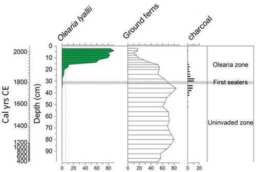
Table 26. Selected examples of islands or island groups in different oceans where pollen-analytical studies show compositional stability prior to the onset of human impact and ecosystem modification. The approximate duration of the periods with stable pollen composition is given, along with the age for the onset of human activities and an indication of plant extinctions or exterminations of all types on each island. The duration of the stable phases are minimal as the pollen assemblages in some of the sequences may commence within the stable phase.

Island or island group	Approx. duration of stable pollen composition (cal. yrs)	Onset of human impact	Extinctions or exterminations (all types)	References
Atlantic Ocean
Iceland	6000	870 CE	-	Caseldine et al. (2003); Lawson et al. (2007)
Færoe Islands	9000	700 CE	+	Jóhansen (1968, 1985, 1989); Hannon and Bradshaw (2000); Hannon et al. (2001, 2005, 2010); Lawson et al. (2005, 2008); Vickers et al. (2005)
Shetland Isles	6000	2500 BCE	+	Jóhansen (1975); Bennett et al. (1992)
Outer Hebrides	8000	500 CE	+	Bennett et al. (1990)
Azores	5500	1450 CE	+	Connor et al. (2012); Rull et al. (2017a)
Canary Isles	7000	100 CE	+	de Nascimento et al. (2009, 2016); Nogué et al. (2013)
Santo Antâo Island, Cabo Verde	~1700	450 CE		Castilla-Beltrán et al. (2019)
Bermuda	8000	1600 CE	-	Watts and Hansen (1986); Rueger and von Wallmenich (1996)
Haiti	6000	3000 BCE	+	Higuera-Gundy et al. (1999)
Tristan da Cunha	5000	1550 CE	-	Hafsten (1960); Ljung (2007); Ljung and Björck (2011)
Inaccessible Island	8000	?	-	Preece et al. (1986)
Nightingale Island	~8000	1700 CE	-	Hafsten (1951)
Gough Island	~4000	1700 CE	-	Hafsten (1960)
Falkland Islands	7000	?	-	Barrow (1978)
South Georgia	6000	?	-	Barrow (1978, 1983a, 1983b); Barrow and Lewis (1983); Clapperton et al. (1989)
South Shetland Islands	300	?	-	van der Knaap and van Leeuwen (1993)
Mediterranean
Balearic Islands	4000	4000 BCE	-	Yll et al. (1994, 1997); Pérez-Obiol and Sadori (2007)
Corsica	4000	2000 BCE	-	Reille (1975)
Sicily	6000	750 BCE	-	Pérez-Obiol and Sadori (2007); Noti et al. (2009); Tinner et al. (2009)
Malta	3000	7500 BCE	-	Carroll et al. (2012)
Crete	3000	6000 BCE	-	Bottema (1980); Bottema and Sarpaki (2003)
Indian Ocean
Madagascar	3000–6000	0–30 CE	+	Burney (1987a, 1993); Virah-Sawmy et al. (2010)
Mauritius	7500	1600 CE	+	de Boer et al. (2013a, 2013b); Gosling et al. (2017)
Marion Island	6000	?	-	Scott (1985)
Pacific Ocean
Carlisle Island, Alaska	7300	?	-	Kuzmicheva et al. (2019)
St Paul Island, Alaska	14,000	?	-	Graham RW et al. (2016); Wang Y et al. (2017); Wooller et al. (2018)
Hawaiian Islands	6000	1000 CE	+	Selling (1948); Burney et al. (1995); Hotchkiss S and Juvik (1999); Hotchkiss S (2003)
Galápagos	9000	500 CE	-	Colinvaux and Schofield (1976); Restrepo et al. (2012); Astudillo (2018)
Marquesas Islands, French Polynesia	1000	1500 CE	-	Allen MS et al. (2011)
Mo’orea, French Polynesia	2000	1000 CE	-	Stevenson et al. (2017)
Tahiti, French Polynesia	>6000	1700 CE	-	Prebble et al. (2016)
Rimatara, French Polynesia	800	1100 CE	+	Prebble and Wilmshurst (2009)
Rapa Nui (Easter Island)	22,000	1200 CE	+	Flenley et al. (1991); Dumont et al. (1998); Hunt TL and Lipo (2006); Mann DG et al. (2008)
Selkirk Island (Chile)	7000	1500 CE	-	Haberle (2003)
Southern Ocean
North Island, New Zealand	2000	1100 CE	-	Prebble and Wilmshurst (2009)
South Island, New Zealand	3000	400 CE	-	Prebble and Wilmshurst (2009)
Tasmania	8000	1400 BCE	-	Fletcher and Thomas (2010); Fletcher et al. (2014a); Stahle et al. (2016); Jones PJ et al. (2017)

- = no evidence of extinctions/exterminations; + = evidence of extinctions/exterminations; ? = unknown or not clear, cal = calibrated

Figure 23. Summary percentage pollen diagram from Ewing Island (sub-Antarctic Auckland Islands) with selected taxa plotted against depth with a calibrated age scale in years CE. Grey zone shows the time of earliest sealing activity in the region. Redrawn from Wilmshurst et al. (2015).

Figure 24. Mount Roraima, a spectacular tepui in Venezuela. Photograph MM from Switzerland (Wikimedia Commons).

Figure 25. Near the summit area of the Eruoda tepui, north-east of the Chimautá massif, Guyana Highlands where Nogué et al. (2009) prepared a pollen sequence covering the last 13,000 years. Photo: Sandra Nogué-Bosch.

Figure 26. Summary pollen and Sporormiella-type (Sporor.) spore stratigraphies (expressed as percentages of upland pollen sum) and charcoal concentrations at Appleman Lake, Indiana between 16,700 and 9000 years ago. The shaded part indicates when the pollen assemblage has no modern pollen analogue. The Sporormiella-type spore record is used as a proxy for megafaunal abundance. Modified from Gill et al. (2009).

Figure 27. Conceptual model of top-down drivers of Late Quaternary vegetation dynamics mediated by biotic interaction. Arrow thickness reflects the hypothesised relative importance of each link. Dashed arrows represent poorly understood or studied relationships. Modified from Gill (2014).

Table 27. Recent contributions to the debate about the causes of Late Pleistocene and early-Holocene megafaunal extinctions.

Barnosky et al. (2004a, 2004b, 2015)	Sandom et al. (2014a)	Westaway et al. (2017)
Koch PL and Barnosky (2006)	Cooper et al. (2015)	Galetti et al. (2018)
Hansen and Galetti (2009)	Grayson and Meltzer (2015)	Price et al. (2018)
Lorenzen et al. (2011)	Graham RW et al. (2016)	Mann DH et al. (2019)
MacDonald et al. (2012)	Saltré et al. (2016)	Smith FA et al. (2019)
	Di Febbraro et al. (2017)

Figure 28. Schematic summaries of the general major trends in the four types of diversity proposed by McGill et al. (2015) at the meta-community scale of organisation (sensu McGill et al. 2015) within the protocratic, mesocratic, Homo sapiens, and oligocratic phases of the Holocene and the last 200 years ('Anthropocene' and 'Great acceleration') based on terrestrial palynological data from northern and central Europe. The vertical axis for all four diversity types runs from low (L) to high (H). The horizontal axis for the four phases and the last 200 years reflects time from oldest (left) to youngest (right). The trends are schematic trajectories of diversity change with the arrows representing the end-point in the different phases. Redrawn from Birks HJB et al. (2016a).

Birks HJB, Berglund BE. 2018. One hundred years of Quaternary pollen analysis 1916–2016. Veg Hist Archaeobot. 27(2):271–309.

 Web of Science ®Google Scholar

Huntley B, Webb T, editors. 1988. Vegetation history. Dordrecht: Kluwer Academic Publishers.

 Google Scholar

Tallis JH. 1991. Plant community history. London: Chapman and Hall.

 Google Scholar

Flenley JR. 1979. The Equatorial Rain Forest: a geological history. London: Butterworth.

 Google Scholar

Bush MB, Flenley JR, Gosling WD, editors. 2011. Tropical rainforest responses to climatic change. 2nd ed. Berlin: Springer.

 Google Scholar

Ritchie JC. 1984. Past and Present Vegetation of the Far Northwest of Canada. Toronto: University of Toronto Press.

 Google Scholar

Ritchie JC. 2008. Postglacial Vegetation of Canada. Cambridge: Cambridge University Press.

 Google Scholar

Webb T, Cushing EJ, Wright HE. 1983a. Holocene changes in the vegetation of the Midwest. In: Wright HE, editor. Late-Quaternary environments of the United States volume 2: the holocene. Minneapolis: University of Minnesota Press; p. 142–165.

 Google Scholar

Davis MB. 1983b. Holocene vegetational history of the eastern United States. In: Wright HE, editor. Late-Quaternary environments of the United States, volume 2: the Holocene. Minneapolis: University of Minnesota Press; p. 166–181.

 Google Scholar

Webb T. 1988a. Eastern North America. In: Huntley B, Webb T, editors. Vegetation history. Dordrecht: Kluwer Academic Publishers; p. 385–414.

 Google Scholar

Grimm EC, Jacobson GL. 2004. Late-Quaternary vegetation history of the eastern United States. In: Gillispie AL, Porter SC, Atwater BF, editors. The Quaternary period in the United States. Amsterdam: Elsevier; p. 381–402.

 Google Scholar

Urrego DH, Bush MB, Silman MR, Correa-Metrio AY, Ledru M-P, Mayle FE, Paduano G, Valencia BG. 2009. Millennial-scale ecological changes in tropical South America since the Last Glacial Maximum. In: Vimeux F, Sylvestre F, Khodri M, editors. Past climate variability in South America and surrounding regions: from the last glacial maximum to the Holocene. Dordrecht: Springer Netherlands; p. 283–300.

 Google Scholar

Huntley B. 1988. Europe. In: Huntley B, Webb T, editors. Vegetation history. Dordrecht: Kluwer; p. 341–383.

 Google Scholar

Firbas F. 1949. Spätz und Nacheiszeitiliche Waldgeschichte Mitteleuropas Nördlich der Alpen. I. Jena: Gustav Fischer.

 Google Scholar

Lang G. 1992. Some aspects of European late- and post-glacial flora history. Acta Botan Fenni. 144:1–17.

 Google Scholar

Lang G. 1994. Quartäre Vegetationsgeschichte Europas. Jena: Gustav Fischer Verlag.

 Google Scholar

Kuneš P, Abraham V. 2017. History of Czech vegetation since the Late Pleistocene. In: Chytrý M, Danihelka J, Kaplan Z et al., editors, pp. 193-227. Flora and vegetation of the Czech Republic. Cham: Springer.

 Google Scholar

Iversen J. 1967. Naturens Udvikling siden sidste Istid. Danmarks Natur. 1:345–445.

 Google Scholar

Iversen J. 1973. The development of Denmark’s nature since the last glacial. Danmarks Geol Unders V. 7-C:1–126 (English translation of Iversen 1967).

 Google Scholar

Godwin H. 1975. The history of the British Flora. A factual basis for phytogeography. 2nd ed. Cambridge: Cambridge University Press.

 Google Scholar

Edwards KJ, Bennett KD, Davies AL. 2018. Palaeoecological perspectives on Holocene environmental change in Scotland. Earth Environ Sci Trans R Soc Edinburgh. 10.1017/S1755691018000208.

 Web of Science ®Google Scholar

West RG. 1964. Inter-relations of ecology and Quaternary palaeobotany. J Ecol. 52(Suppl):47–57.

 Google Scholar

Walker D. 1982a. Vegetation’s fourth dimension. New Phytol. 90(3):419–429.

 Google Scholar

Walker D. 1990. Purpose and method in Quaternary palynology. Rev Palaeobot Palynol. 64(1–4):13–27.

 Web of Science ®Google Scholar

Birks HJB. 1986. Late Quaternary biotic changes in terrestrial and limnic environments, with particular reference to north west Europe. In: Berglund BE, editor. Handbook of Holocene palaeoecology and palaeohydrology. Chichester: J Wiley & Sons; p. 3–65.

 Google Scholar

Birks HJB. 1993a. Quaternary paleoecology and vegetation science - current contributions and possible future developments. Rev Palaeobot Palynol. 79(1–2):153–177.

 Web of Science ®Google Scholar

Bennett KD. 1988b. Post-glacial vegetation history: ecological considerations. In: Huntley B, Webb T, editors. Vegetation history. Dordrecht: Kluwer; p. 699–774.

 Google Scholar

Davis MB. 1989c. Retrospective studies. In: Likens GE, editor. Long-term studies in ecology: approaches and alternatives. New York: Springer; p. 71–89.

 Google Scholar

Foster DR, Schoonmaker PK, Pickett STA. 1990. Insights from paleoecology to community ecology. Trends Ecol Evol. 5(4):119–122.

 PubMed Web of Science ®Google Scholar

Delcourt HR, Delcourt PA. 1991. Quaternary ecology. A paleoecological perspective. London: Chapman & Hall.

 Google Scholar

Ritchie JC. 1991. Paleoecology: status and prospect. In: Shane LCK, Cushing EJ, editors. Quaternary landscapes. Minneapolis: University of Minnesota Press; p. 113–128.

 Google Scholar

Ritchie JC. 1995. Current trends in studies of long-term plant community dynamics. New Phytol. 130:469–494.

 PubMed Web of Science ®Google Scholar

Schoonmaker PK, Foster DR. 1991. Some implications of paleoecology for contemporary ecology. Bot Rev. 57(3):204–245.

 Web of Science ®Google Scholar

Huntley B. 1996. Quaternary palaeoecology and ecology. Quat Sci Rev. 15:591–606.

 Web of Science ®Google Scholar

Mitchell FJG. 2011. Exploring vegetation in the fourth dimension. Trends Ecol Evol. 26(1):45–52.

 Web of Science ®Google Scholar

Luouys J, Wilkinson DM, Bishop LC. 2012. Ecology needs a paleontological perspective. In: Louys J, editor. Paleontology in ecology and conservation. Berlin: Springer-Verlag; p. 23–38.

 Google Scholar

Reitalu T, Kunes P, Giesecke T. 2014. Closing the gap between plant ecology and Quaternary palaeoecology. J Veg Sci. 25:1188–1194.

 Web of Science ®Google Scholar

Jackson ST, Blois JL. 2015. Community ecology in a changing environment: Perspectives from the Quaternary. Proc Natl Acad Sci USA. 112(16):4915–1921.

 PubMed Web of Science ®Google Scholar

Nogués-Bravo D, Rodríguez-Sánchez F, Orsini L, de Boer E, Jansson R, Morlon H, Fordham DA, Jackson ST. 2018. Cracking the code of biodiversity responses to past climate change. Trends Ecol Evol. 33(10):765–776.

 Web of Science ®Google Scholar

Walker D. 1982b. The development of resilience in burned vegetation. In: Newman EI, editor. Plant community as a working mechanism. Oxford: Blackwell Scientific Publications; p. 27–43.

 Google Scholar

Walker D. 1989. Diversity and stability. In: Cherrett JM, Bradshaw AD, Goldsmith FB et al., editors. Ecological concepts. Oxford: Blackwell; p. 115–145.

 Google Scholar

Davis MB. 1986a. Climatic instability, time lags, and community disequilibrium. In: Diamond J, Case TJ, editors. Community Ecology. New York: Harper & Row; p. 269–284.

 Google Scholar

Walker D, Chen Y. 1987. Palynological light on tropical forest dynamics. Quat Sci Rev. 6:77–82.

 Web of Science ®Google Scholar

Prentice IC. 1988a. Paleoecology and plant-population dynamics. Trends Ecol Evol. 3:343–345.

 PubMed Web of Science ®Google Scholar

Bennett KD. 1997. Evolution and ecology: the pace of life. Cambridge: Cambridge University Press.

 Google Scholar

Iversen J. 1958. The bearing of glacial and interglacial epochs on the formation and extinction of plant taxa. Syst Today Uppsala Univ Årsskr 6:210–215.

 Google Scholar

Andersen ST. 1994. History of the terrestrial environment in the Quaternary of Denmark. Bull Geol Soc Den. 41:219–228.

 Web of Science ®Google Scholar

Birks HJB, Birks HH. 2004. The rise and fall of forests. Science. 305(5683):484–485.

 PubMed Web of Science ®Google Scholar

de Beaulieu J-L, Andrieu-Ponel V, Reille M, Grüger E, Tzedakis C, Svitavská Svobodova H. 2001. An attempt at correlation between the Velay pollen sequence and the Middle Pleistocene stratigraphy from central Europe. Quat Sci Rev. 20(16):1593–1602.

 Web of Science ®Google Scholar

de Beaulieu J-L, Andrieu-Ponel V, Cheddadi R, Guiter F, Ravazzi C, Reille M, Rossi S. 2006. Apport des longues séquences lacustres à la connaissance des variations des climats et des paysages pléistocènes. Comptes Rendus Palevol. 5(1):65–72.

 Google Scholar

Willis KJ, Braun M, Sumegi P, Toth A. 1997. Does soil change cause vegetation change or vice versa? A temporal perspective from Hungary. Ecology. 78(3):740–750.

 Web of Science ®Google Scholar

Ammann B, Oldfield F, editors. 2000. Rapid warming project. Palaeogeogr Palaeoclimatol Palaeoecol. 159:191–366.

 Web of Science ®Google Scholar

Ammann B, van Leeuwen JFN, van der Knaap WO, Lischke H, Heiri O, Tinner W. 2013a. Vegetation responses to rapid warming and to minor climatic fluctuations during the Late-Glacial Interstadial (GI-1) at Gerzensee (Switzerland). Palaeogeogr Palaeoclimatol Palaeoecol. 391:40–59.

 Web of Science ®Google Scholar

Ammann B, van Raden UJ, Schwander J, Eicher U, Gilli A, Bernasconi SM, van Leeuwen JFN, Lischke H, Brooks SJ, Heiri O et al. 2013b. Responses to rapid warming at Termination 1a at Gerzensee (central Europe): primary succession, albedo, soils, lake development, and ecological interactions. Palaeogeogr Palaeoclimatol Palaeoecol. 391:111–131.

 Web of Science ®Google Scholar

Ammann B, von Grafenstein U, van Raden UJ. 2013c. Biotic responses to rapid warming about 14,685yr BP: introduction to a case study at Gerzensee (Switzerland). Palaeogeogr Palaeoclimatol Palaeoecol. 391:3–12.

 Web of Science ®Google Scholar

Birks HJB, Birks HH, Ammann B. 2016b. The fourth dimension of vegetation. Science. 354:412–413.

 PubMed Web of Science ®Google Scholar

Harley JL, Harley EL. 1987. A check-list of mycorrhiza in the British flora. New Phytol. 105 (suppl.):1–102.

 PubMed Web of Science ®Google Scholar

Read DJ. 1993a. Mycorrhiza in plant communities. Mol Plant Pathol. 9:1–31.

 Google Scholar

Read DJ. 1993b. Plant-microbe mutualism and community structure. In: Schulze E-D, Mooney HA, editors. Biodiversity and ecosystem function. Berlin: Springer; p. 181–209.

 Google Scholar

Cázares E, Trappe JM, Jumpponen A. 2005. Mycorrhiza-plant colonization patterns on a subalpine glacier foreland as a model system of primary succession. Mycorrhiza. 15:405–416.

 PubMed Web of Science ®Google Scholar

Kuneš P, Odgaard BV, Gaillard MJ. 2011. Soil phosphorus as a control of productivity and openness in temperate interglacial forest ecosystems. J Biogeogr. 38:2150–2164.

 Web of Science ®Google Scholar

Dickie IA, Martinez-Garciá LB, Koele N, Grelet G-A, Tylianakis JM, Peltzer DA, Richardson SJ. 2013. Mycorrhizas and mycorrhizal fungal communities throughout ecosystem development. Plant Soil. 367:11–39.

 Web of Science ®Google Scholar

Iversen J. 1954. The Late-glacial flora of Denmark and its relation to climate and soil. Danmarks Geol Unders II. 80:87–119.

 Google Scholar

Andersen ST. 1961. Vegetation and its environment in Denmark in the Early Weichselian Glacial (Last Glacial). Danmarks Geol Unders II. 75:1–175.

 Google Scholar

Birks HJB. 1973. Past and Present Vegetation of the Isle of Skye - A Palaeoecological Study. Cambridge: Cambridge University Press.

 Google Scholar

Fries M. 1967. Lennart von Post’s pollen diagram series of 1916. Rev Palaeobot Palynol. 4:9–13.

 Google Scholar

von Post L. 1924. Ur de sydsvenska skogarnas regionala historia under post-arktisk tid. Geologiska Föreningens i Stockholm Förhandlingar. 46:83–128.

 Google Scholar

von Post L. 1926a. Einige Aufgaben der regionalen Moorforschung. Sveriges Geol Undersökning Ser C. 337:1–41.

 Google Scholar

Huntley B, Birks HJB. 1983. An atlas of past and present pollen maps for europe: 0-13000 years ago. Cambridge: Cambridge University Press.

 Google Scholar

Brewer S, Giesecke T, Davis BAS, Finsinger W, Wolters S, Binney HA, de Beaulieu JL, Fyfe R, Gil-Romera G, Kühl N et al. 2017. Late-glacial and Holocene European pollen data. J Maps. 13(2):921–928.

 Web of Science ®Google Scholar

Moran JM. 1973. The late-glacial retreat of ‘Arctic’ air as suggested by the onset of Picea decline. Prof Geogr. 25:373–376.

 Web of Science ®Google Scholar

Davis MB. 1976. Pleistocene biogeography of temperate deciduous forests. Geosci Man. 13:13–26.

 Google Scholar

Davis MB. 1978. Climatic interpretation in Quaternary sediments. In: Walker D, Guppy JC, editors. Biology and Quaternary environments. Canberra: Australian Academy of Science; p. 35–51.

 Google Scholar

Davis MB. 1983a. Quaternary history of deciduous forests of eastern North America and Europe. Ann Missouri Bot Garden. 70:550–563.

 Web of Science ®Google Scholar

Bernabo JC, Webb T. 1977. Changing patterns in the Holocene pollen record of northeastern North America: a mapped summary. Quat Res. 8:64–96.

 Web of Science ®Google Scholar

Jacobson GL. 1979. The palaeoecology of white pine (Pinus strobus) in Minnesota. J Ecol. 67(2):697–726.

 Web of Science ®Google Scholar

Webb T. 1981. The past 11000 years of vegetational change in eastern North America. BioScience. 31:501–506.

 Web of Science ®Google Scholar

Webb T, Richard PH, Mott RJ. 1983b. A mapped history of Holocene vegetation in southern Quebec. Syllogeus. 49:273–336.

 Google Scholar

Björck S. 1985. Deglaciation chronology and revegetation in northwestern Ontario. Can J Earth Sci. 22:850–871.

 Web of Science ®Google Scholar

Davis RB, Jacobson GL. 1985. Late glacial and early Holocene landscapes in northern New England and adjacent areas of Canada. Quat Res. 23:341–368.

 Web of Science ®Google Scholar

Gaudreau DC, Webb T. 1985. Late-Quaternary pollen stratigraphy and isochrone maps for the northeastern United States. In: Bryant VM, Holloway RG, editors. Pollen records of Late-Quaternary sediments. Dallas: American Association of Stratigraphic Palynologists Foundation; p.245–280.

 Google Scholar

Davis MB, Woods KD, Webb SL, Futyma RP. 1986. Dispersal versus climate: expansion of Fagus and Tsuga into the Upper Great Lakes region. Vegetatio. 67:93–103.

 Google Scholar

Birks HJB. 1989. Holocene isochrone maps and patterns of tree-spreading in the British Isles. J Biogeogr. 16(6):503–540.

 Web of Science ®Google Scholar

Donner JJ. 1963. The zoning of the post-glaial pollen diagrams in Finland and the main changes in the forest composition. Acta Botan Fenni. 65:2–40.

 Google Scholar

Aario R. 1965. Die Fichtenverhäufigung in Lichte von C14-bestimmungen und die Altersverhaltnisse der Finnischen pollenzonen. C R Soc Géol Finlande. 37:215–231.

 Google Scholar

Aartolahti T. 1966. Über die Einwanderlung und die Verhäufigung der Fichte in Finnland. Ann Bot Fennici. 3:368–379.

 Google Scholar

Aartolahti T. 1967. Zur Rationellen Tilia-pollengrenze (To) in Finnland. Fennia. 97:1–30.

 Google Scholar

Moe D. 1970. Post-glacial immigration of Picea abies into Fennoscandia. Bot Notiser. 123 (1):61–66.

 Web of Science ®Google Scholar

Persson C. 1975. Speculations on the immigration of spruce in Sweden. Geologiska Föreningens i Stockholm Förhandlingar. 97:292–294.

 Google Scholar

Tolonen K, Ruuhijärvi R. 1976. Standard pollen diagrams from the Salpausoelkä region of southern Finland. Ann Bot Fennici. 13:155–196.

 Google Scholar

Høeg HI. 1978. The immigration of Picea abies to southeasten Norway with special regard to Telemark (a preliminary report). Norw J Bot. 25:19–21.

 Google Scholar

Tolonen K. 1983. Kuusen levinneisyy historiaa suomessa. Sorbifolia. 14:53–58.

 Google Scholar

Serebryanny LR. 1971. Dinamika rasprostraneniia nekotoryh drevesnyn porod na severo-zapade SSR v poslelednikovoe vremia. In: Neustadt MI, editor. Palinologiia golotsena. Moscow: Nauka; p. 17–31.

 Google Scholar

Serebryanny LR. 1973. Post-glacial migration rates of tree species in the northwestern regions of the USSR: palynology and radiocarbon dating. In: Khotinsky NA, Koreneva EV, editors. Palynology: holocene and marine palynology. Moscow: Nauka; p. 14–18.

 Google Scholar

Feurdean A, Bhagwat SA, Willis KJ, Birks HJB, Lischke H, Hickler T. 2013. Tree migration-rates: narrowing the gap between inferred post-glacial rates and projected rates. PLoS One. 8(8):e71797.

 PubMed Web of Science ®Google Scholar

Giesecke T, Brewer S. 2018. Notes on the post-glacial spread of abundant European tree taxa. Veg Hist Archaeobot. 27(2):337–349.

 Web of Science ®Google Scholar

Davis MB. 1987. Invasions of forest communities during the Holocene: beech and hemlock in the Great Lakes region. In: Gray AJ, Crawley MJ, Edwards PJ, editors. Colonization, Succession and Stability. Oxford: Blackwell Scientific Publishing; p. 373–393.

 Google Scholar

Giesecke T. 2013. Changing plant distributions and abundances. In: Elias SA, editor. Encyclopedia of Quaternary science. Amsterdam: Elsevier; p. 854–860.

 Google Scholar

Tinner W, Lotter AF. 2006. Holocene expansions of Fagus sylvatica and Abies alba in central Europe: Where are we after eight decades of debate? Quat Sci Rev. 25:526–549.

 Web of Science ®Google Scholar

Jackson ST, Booth RK. 2002. The role of late Holocene climate variability in the expansion of yellow birch in the western Great Lakes region. Divers Distrib. 8:275–284.

 Web of Science ®Google Scholar

Krause TR, Whitlock C. 2017. Climatic and non-climatic controls shaping early postglacial conifer history in the northern Greater Yellowstone Ecosystem, USA. J Quat Sci. 32(7):1022–1036.

 Web of Science ®Google Scholar

Woods KD, Davis MB. 1989. Paleoecology of range limits: beech in the Upper Peninsula of Michigan. Ecology. 70:681–696.

 Web of Science ®Google Scholar

Parshall T. 2002. Late Holocene stand-scale invasion by hemlock (Tsuga canadensis) at its western range limit. Ecology. 83(5):1386–1398.

 Web of Science ®Google Scholar

Booth RK, Jackson ST, Gray CED. 2004. Paleoecology and high-resolution paleohydrology of a kettle peatland in upper Michigan. Quat Res. 61:1–13.

 Web of Science ®Google Scholar

Minckley TA, Booth RK, Jackson ST. 2011. Response of arboreal pollen abundance to late-Holocene drought events in the Upper Midwest, USA. Holocene. 22(5):531–539.

 Web of Science ®Google Scholar

Clifford MJ, Booth RK. 2015. Late-Holocene drought and fire drove a widespread change in forest community composition in eastern North America. Holocene. 25(7):1102–1110.

 Web of Science ®Google Scholar

Lyford ME, Jackson ST, Betancourt JL, Gray ST. 2003. Influence of landscape structure and climate variability on a late Holocene plant migration. Ecol Monogr 73:567–583.

 Web of Science ®Google Scholar

Peñalba MC, Payette S. 1997. Late-Holocene expansion of eastern larch (Larix laricina [Du Roi] K. Koch) in northwestern Québec. Quat Res. 48(1):114–121.

 Web of Science ®Google Scholar

Edwards ME, Franklin-Smith L, Clarke C, Baker J, Hill S, Gallagher K. 2015. The role of fire in the mid-Holocene arrival and expansion of lodgepole pine (Pinus contorta var. latifolia Engelm. ex S. Watson) in Yukon Holocene. 25(1):64–78.

 Web of Science ®Google Scholar

Gray ST, Betancourt JL, Jackson ST, Eddy RG. 2006. Role of multidecadal climatic variability in a range extension of pinyon pine. Ecology. 87(5):1124–1130.

 PubMed Web of Science ®Google Scholar

Anderson RS, Kaufman DS, Berg E, Schiff C, Daigle T. 2017. Holocene biogeography of Tsuga mertensiana and other conifers in the Kenai Mountains and Prince William Sound, south-central Alaska. Holocene. 27(4):485–495.

 Web of Science ®Google Scholar

Magri D, Vendramin GG, Comps B, Dupanloup I, Geburek T, Gömöry D, Latałowa M, Litt T, Paule L, Roure JM et al. 2006. A new scenario for the Quaternary history of European beech populations: palaeobotanical evidence and genetic consequences. New Phytol. 171:199–221.

 PubMed Web of Science ®Google Scholar

Lindner L, Morks S, Nita M. 2013. Climatostratigraphy of interglacials in Poland: Middle and Upper Pleistocene lower boundaries from a Polish perspective. Quatern Int. 292:113–123.

 Web of Science ®Google Scholar

Stachowicz-Rybka R. 2015a. Environmental and climate changes reflected in the Domuraty 2 section (NE Poland) based on analysis of plant macroremains. Acta Palaeobot. 55(2):213.

 Google Scholar

Mamakowa K, Velichkevich FY. 1993a. Aracites interglacialis Wieliczk. - extinct plant found in the floras of the Mazovian (Alexandrian, Likhvinian) interglacial in Poland, Belarus, Russia, and the Ukraine. Acta Palaeobot. 33(2):321–341.

 Google Scholar

Velichkevich FY, Granoszewski W. 1996. Potamogeton sukaczevii Wieliczk. in the NeoPleistocene floras of Poland, Belarus and Lithuania. Acta Palaeobot. 36(1):97–105.

 Google Scholar

Velichkevich FY, Lesiak MA. 1996. Fossil Potamogeton species of Mizerna. Acta Palaeobot. 36(1):79–95.

 Google Scholar

Velichkevich FY, Mamakowa K. 2003. Revision of plant macrofossils from the Mazovian interglacial locality Nowiny Żukowskie (SE Poland). Acta Palaeobot. 43(1):61–76.

 Google Scholar

Velichkevich FY, Zastawniak E. 2003. The Pliocene flora of Kholmech, south-eastern Belarus and its correlation with other Pliocene floras of Europe. Acta Palaeobot. 43(2):137–259.

 Google Scholar

Velichkevich FY, Mamakowa K, Stuchlik L. 2004. Revision of some Mazovian interglacial macrofossil floras of Poland. Acta Palaeobot. 44(1):93–104.

 Google Scholar

Stachowicz-Rybka R. 2011. Flora and vegetation changes on the basis of plant macroremains analysis from an early Pleistocene lake of the Augustów Plain, NE Poland. Acta Palaeobot. 51:39–103.

 Google Scholar

Stachowicz-Rybka R. 2015b. Record of environmental and climatic changes in middle Pleistocene sediments from Łuków (eastern Poland) on the basis of plant macroremains analysis. Acta Palaeobot. 55(1):68.

 Google Scholar

Stachowicz-Rybka R. 2015c. Vegetation of the Ferdynandovian interglacial (MIS 13–15) based on plant macrofossils from a new profile of the stratotype site. Acta Palaeobot. 55(2):233.

 Google Scholar

Drzymulska D. 2018. On the history of Brasenia Schreb. in the European Pleistocene. Veg Hist Archaeobot. 27(3):527–534.

 Web of Science ®Google Scholar

Svenning J-C. 2003. Deterministic Plio-Pleistocene extinctions in the European cool-temperate tree flora. Ecol Lett. 6:646–653.

 Web of Science ®Google Scholar

Tralau H. 1959. Extinct aquatic plants of Europe. Bot Notiser. 112(4):385–406.

 Google Scholar

Tralau H. 1963a. Asiatic Dicotyledonous affinities in the Cainozoic flora of Europe. Kungliga Sven Vetenskapsakademiens Handlingar. 9:7–87.

 Google Scholar

van der Hammen T, Wijmstra TA, Zagwijn WH. 1971. The floral record of the Late Cenozoic of Europe. In: Turekian KK, editor. The Late Cenozoic Glacial ages. New Haven: Yale University Press; p. 391–424.

 Google Scholar

Huckerby E, Oldfield F. 1976. The Quaternary vegetational history of the French Pays Basque, II: Plant macrofossils and additional pollen-analytical data. New Phytol. 77:499–526.

 Web of Science ®Google Scholar

Watts WA. 1988. Europe. In: Huntley B, Webb T, editors. Vegetation history. Dordrecht: Kluwer; p. 155–192.

 Google Scholar

Mai DH. 1995. Tertiäre Vegetationsgeschichte Europas. Jena: Gustav Fischer Verlag.

 Google Scholar

Góis-Marques CA, Mitchell RL, de Nascimento L, Fernández-Palacios JM, Madeira J, Menezes de Sequeira M. 2019. Eurya stigmosa (Theaceae), a new and extinct record for the Calabrian stage of Madeira Island (Portugal): 40Ar/39Ar dating, palaeoecological and oceanic island palaeobiogeographical implications. Quat Sci Rev. 206:129–140.

 Web of Science ®Google Scholar

Holt RD. 1990. The microevolutionary consequences of climate change. Trends Ecol Evol. 5(9):311–315.

 PubMed Web of Science ®Google Scholar

Nicotra AB, Atkin OK, Bonser SP, Davidson AM, Finnegan EJ, Mathesius U, Poot P, Purugganan MD, Richards CL, Valladares F et al. 2010. Plant phenotypic plasticity in a changing climate. Trends Plant Sci. 15(12):684–692.

 PubMed Web of Science ®Google Scholar

Merilä J, Hendry AP. 2014. Climate change, adaptation, and phenotypic plasticity: the problem and the evidence. Evol Appl. 7(1):1–14.

 PubMed Web of Science ®Google Scholar

Davis MB, Shaw RG. 2001. Range shifts and adaptive responses to Quaternary climate change. Science. 292(5517):673–679.

 PubMed Web of Science ®Google Scholar

Sussman R. 2010. The Oldest Things in the World. Chicago: University of Chicago Press.

 Google Scholar

Etterson JR, Franks SJ, Mazer SJ, Shaw RG, Gorden NLS, Schneider HE, Weber JJ, Winkler KJ, Weis AE. 2016. Project baseline: An unprecedented resource to study plant evolution across space and time. Am J Bot. 103(1):164–173.

 PubMed Web of Science ®Google Scholar

Etterson JR, Shaw RG. 2001. Constraint to adaptive evolution in response to global warming. Science. 294(5540):151–154.

 PubMed Web of Science ®Google Scholar

Dawson TP, Jackson ST, House JI, Prentice IC, Mace GM. 2011. Beyond predictions: biodiversity conservation in a changing climate. Science. 332:53–58.

 PubMed Web of Science ®Google Scholar

Graae BJ, Vandvik V, Armbruster WS, Eiserhardt WL, Svenning J-C, Hylander K, Ehrlén J, Speed JDM, Klanderud K, Bråthen KA et al. 2018. Stay or go – how topographic complexity influences alpine plant population and community responses to climate change. Perspect Plant Ecol Evol Syst. 30:41–50.

 Web of Science ®Google Scholar

Davis MB, Shaw RG, Etterson JR. 2005. Evolutionary responses to changing climate. Ecology 86(7):1704–1714.

 Web of Science ®Google Scholar

Hill JK, Griffiths HM, Thomas CD. 2011. Climate change and evolutionary adaptations at species’ range margins. Annu Rev Entomol. 56(1):143–159.

 PubMedGoogle Scholar

Henn JJ, Buzzard V, Enquist BJ, Halbritter AH, Klanderud K, Maitner BS, Michaletz ST, Pötsch C, Seltzer L, Telford RJ et al. 2018. Intraspecific trait variation and phenotypic plasticity mediate alpine plant species response to climate change. Front Plant Sci. 9(1548).

 PubMed Web of Science ®Google Scholar

Jump AS, Peñuelas J. 2005. Running to stand still: adaptation and the response of plants to rapid climate change. Ecol Lett. 8(9):1010–1020.

 PubMed Web of Science ®Google Scholar

Hoffmann AA, Sgrò CM. 2011. Climate change and evolutionary adaptation. Nature. 470:479–485.

 PubMed Web of Science ®Google Scholar

Lallensack R. 2018. Evology. Nature. 554:19–21.

 Web of Science ®Google Scholar

Parmesan C. 2006. Ecological and evolutionary responses to recent climate change. Annu Rev Ecol Evol Syst. 37(1):637–669.

 Web of Science ®Google Scholar

Shaw RG, Etterson JR. 2012. Rapid climate change and the rate of adaptation: insight from experimental quantitative genetics. New Phytol. 195(4):752–765.

 Web of Science ®Google Scholar

Aitken SN, Yeaman S, Holliday JA, Wang T, Curtis-McLane S. 2008. Adaptation, migration or extirpation: climate change outcomes for tree populations. Evol Appl. 1(1):95–111.

 PubMed Web of Science ®Google Scholar

Alberto FJ, Aitken SN, Alía R, González-Martínez SC, Hänninen H, Kremer A, Lefèvre F, Lenormand T, Yeaman S, Whetten R et al. 2013. Potential for evolutionary responses to climate change – evidence from tree populations. Glob Chang Biol. 19(6):1645–1661.

 PubMed Web of Science ®Google Scholar

de Witte LC, Stöcklin J. 2010. Longevity of clonal plants: why it matters and how to measure it. Ann Bot. 106(6):859–870.

 PubMed Web of Science ®Google Scholar

Franks SJ, Weber JJ, Aitken SN. 2014. Evolutionary and plastic responses to climate change in terrestrial plant populations. Evol Appl. 7(1):123–139.

 PubMed Web of Science ®Google Scholar

Jackson ST, Overpeck JT. 2000. Responses of plant populations and communities to environmental changes of the late Quaternary. Paleobiology. 26 (Supplement 4): 194–220.

 Web of Science ®Google Scholar

Bartlein PJ, Anderson KH, Anderson PM, Edwards ME, Mock CJ, Thompson RS, Webb RS, Webb T, Whitlock C. 1998. Paleoclimatic simulations for North America over the past 21,000 years: features of the simulated climates and comparisons with paleoenvironmental data. Quat Sci Rev. 17:549–585.

 Web of Science ®Google Scholar

Sandom CJ, Ejrnæs R, Hansen MDD, Svenning J-C. 2014b. High herbivore density associated with vegetation diversity in interglacial ecosystems. Proc Natl Acad Sci USA. 111(11):4162–4167.

 Web of Science ®Google Scholar

Past Interglacials Working Group of PAGES. 2016. Interglacials of the last 800,000 years. Rev Geophys. 54:162–219.

 Web of Science ®Google Scholar

Jackson ST, Webb RS, Anderson KH, Overpeck JT, Webb T, Williams JW, Hansen BCS. 2000b. Vegetation and environment in eastern North America during the last glacial maximum. Quat Sci Rev. 19:489–508.

 Web of Science ®Google Scholar

Jackson ST, Williams JW. 2004. Modern analogs in Quaternary paleoecology: Here today, gone yesterday, gone tomorrow? Annu Rev Earth Planet Sci. 32:495–537.

 Web of Science ®Google Scholar

Cushing EJ. 1963. Late-Wisconsin pollen stratigraphy in east-central Minnesota [PhD thesis]. Minnesota: University of Minnesota.

 Google Scholar

Birks HH. 2003. The importance of plant macrofossils in the reconstruction of Lateglacial vegetation and climate: examples from Scotland, western Norway, and Minnesota, USA. Quat Sci Rev. 22:453–473.

 Web of Science ®Google Scholar

Gill JL, Williams JW, Jackson ST, Lininger KB, Robinson GS. 2009. Pleistocene megafaunal collapse, novel plant communities, and enhanced fire regimes in North America. Science. 326:1100–1103.

 PubMed Web of Science ®Google Scholar

Gill JL, Williams JW, Jackson ST, Donnelly JP, Schellinger GC. 2012. Climatic and megaherbiovry controls on late-glacial vegetation dynamics: a new, high-resolution, multi-proxy record from Silver Lake, Ohio. Quat Sci Rev. 34:66–80.

 Web of Science ®Google Scholar

Jones RA, Williams JW, Jackson ST. 2017. Vegetation history since the last glacial maximum in the Ozark highlands (USA): A new record from Cupola Pond, Missouri. Quat Sci Rev. 170 (SupplementC):174–187.

 Google Scholar

Webb T. 1987. The appearance and disappearance of major vegetational assemblages: Long-term vegetational dynamics in eastern North America. Vegetatio. 69:177–187.

 Google Scholar

Prentice IC. 1983. Postglacial climatic change: vegetation dynamics and the pollen record. Prog Phys Geog. 7(2):273–286.

 Google Scholar

COHMAP Members. 1988. Climatic changes of the last 18,000 years: observations and model simulations. Science. 241:1043–1052.

 PubMed Web of Science ®Google Scholar

Wright HE, Kutzbach JE, Webb T, Ruddiman WF, Street-Perrott FA, Bartlein PJ, editors. 1993. Global climates since the last glacial maximum. Minneapolis: University of Minnesota Press.

 Google Scholar

Birks HJB. 2008. Holocene climate research - progress, paradigms, and problems. In: Battarbee RW, Binney HA, editors. Natural climate variability and global warming: a Holocene perspective. Oxford: Wiley-Blackwell; p. 7–57.

 Google Scholar

Tsukada M, Sugita S. 1982. Late Quaternary dynamics of pollen influx at Mineral Lake, Washington. Bot Mag Tokyo. 95:401–418.

 Web of Science ®Google Scholar

Tsukada M. 1982c. Cryptomeria japonica: Glacial refugia and late-glacial and postglacial migration. Ecology. 63(4):1091–1105.

 Web of Science ®Google Scholar

Tsukada M. 1982d. Late-Quaternary shift of Fagus distribution. Bot Mag Tokyo. 95:203–217.

 Web of Science ®Google Scholar

Bennett KD. 1986. The rate of spread and population increase of forest trees during the Postglacial. Philos Trans R Soc B Bio Sci. 314(1167):523–531.

 Web of Science ®Google Scholar

Bennett KD. 1988a. Holocene geographic spread and population expansion of Fagus grandifolia in Ontario, Canada. J Ecol. 76:547–557.

 Web of Science ®Google Scholar

MacDonald GM, Cwynar LC. 1991. Post-glacial population growth rates of Pinus contorta ssp. latifolia in western Canada. J Ecol. 79:417–429.

 Web of Science ®Google Scholar

MacDonald GM. 1993a. Fossil pollen analysis and the reconstruction of plant invasions. Adv Ecol Res. 24:67–110.

 Web of Science ®Google Scholar

Fuller JL. 1998. Ecological impact of the mid-Holocene hemlock decline in southern Ontario, Canada. Ecology. 79(7):2337–2351.

 Web of Science ®Google Scholar

Bennett KD. 1983. Post-glacial population expansion of forest trees in Norfolk, UK. Nature. 303(5913):164–167.

 Web of Science ®Google Scholar

Giesecke T, Hickler T, Kunkel T, Sykes MT, Bradshaw RHW. 2007. Towards an understanding of the Holocene distribution of Fagus sylvatica L. J Biogeogr. 34:118–131.

 Web of Science ®Google Scholar

Bradshaw RHW, Kito N, Giesecke T. 2010. Factors influencing the Holocene history of Fagus. For Ecol Manage. 259(11):2204–2212.

 Web of Science ®Google Scholar

Magri D. 1989. Interpreting long-term exponential growth of plant populations in a 250,000-year pollen record from Valle di Castiglione (Roma). New Phytol. 112:123–128.

 Web of Science ®Google Scholar

Chen Y. 1988. Early Holocene population expansion of some rainforest trees in the Lake Barrine Basin. Aust J Ecol. 13:225–233.

 Web of Science ®Google Scholar

Tsukada M. 1981. Cryptomeria japonica D. Don I. Pollen dispersal and logistic forest expansion. Jpn J Ecol. 31:371–383.

 Google Scholar

Tsukada M. 1982a. Pseudotsuga menziesii (Mirb.) Franco: its pollen dispersal and late Quaternary history in the Pacific Northwest. Jpn J Ecol. 32:159–187.

 Google Scholar

Tsukada M. 1982b. Late-Quaternary development of the Fagus forest in the Japanese Archipelago. Jpn J Ecol. 32:113–118.

 Google Scholar

Kito N, Takimoto F. 1999. Population growth and migration rate of Fagus crenata during the Holocene in southwestern Hokkaido, Japan. Quat Res. 38:297–311.

 Google Scholar

Peglar SM. 1993a. The mid-Holocene Ulmus decline at Diss Mere, Norfolk, UK: a year-by-year pollen stratigraphy from annual laminations. Holocene. 3 (1):1–13.

 Google Scholar

Peglar SM, Birks HJB. 1993. The mid-Holocene Ulmus fall at Diss Mere, south-east England - disease and human impact? Veg Hist Archaeobot. 2:61–68.

 Google Scholar

Tsukada M. 1983. Late-Quaternary spruce decline and rise in Japan and Sakhalin. Bot Mag Tokyo. 96:127–133.

 Google Scholar

Piñero D, Martinez-Ramos M, Sarukhán J. 1984. A population model of Astrocaryum mexicanum and a sensitivity model of its finite rate of increase. J Ecol. 72:977–991.

 Web of Science ®Google Scholar

Watts WA. 1973. Rates of change and stability in vegetation in the perspective of long periods of time. In: Birks HJB, West RG, editors. Quaternary plant ecology. Oxford: Blackwell Scientific Publications; p. 195–206.

 Google Scholar

Birks HJB, Tinner W. 2016a. European tree dynamics and invasions during the Quaternary. In: Krumm F, Quadt V, editors. Introduced tree species to European forests: challenges and opportunities. Luxembourg: Publication Office of the European Union; p. 21–43.

 Google Scholar

Fægri K, Iversen J. 1950. Text-book of modern pollen analysis. Copenhagen: Munksgaard.

 Google Scholar

Williams JW, Blois JL, Shuman BN. 2011a. Extrinsic and intrinsic forcing of abrupt ecological change: case studies from the late Quaternary. J Ecol. 99:664–677.

 Web of Science ®Google Scholar

Grimm EC. 1983. Chronology and dynamics of vegetation change in the prairie‐woodland region of southern Minnesota, USA New Phytol 93(2):311–350.

 Web of Science ®Google Scholar

Camill P, Umbanhowar CE, Teed R, Geiss CE, Aldinger J, Dvorak L, Kenning J, Limmer J, Walkup K. 2003. Late-glacial and Holocene climatic effects on fire and vegetation dynamics at the prarie–forest ecotone in south-central Minnesota. J Ecol. 91:822–836.

 Web of Science ®Google Scholar

Szeicz JM, Haberle SG, Bennett KD. 2003. Dynamics of North Patagonian reainforests from fine-resolution pollen, charcoal and tree-ring analysis, Chonos Archipelago, southern Chile. Austral Ecol. 28:413–422.

 Web of Science ®Google Scholar

Tausch RJ, Wigand PE, Burkhardt JW. 1993. Plant community thresholds, multiple steady states, and multiple successional pathways: legacy of the Quaternary? J Range Manag. 46(5):439–447.

 Google Scholar

Craine JM, McLauchlan KK. 2004. The influence of biotic drivers on North American palaeorecords: alternatives to climate. Holocene. 14(5):787–791.

 Web of Science ®Google Scholar

Franklin SB, Tolonen M. 2000. Temporally-explicit models of fire and forest. Plant Ecol. 146:145–168.

 Web of Science ®Google Scholar

Umbanhowar CE. 2004. Interaction of fire, climate and vegetation change at a large landscape scale in the Big Woods of Minnesota, USA. Holocene. 14(5):661–676.

 Web of Science ®Google Scholar

Lytle DE. 2005. Palaeoecological evidence of state shifts between forest and barrens on a Michigan sand plain, USA. Holocene. 15:821–836.

 Web of Science ®Google Scholar

Lynch EA, Calcote R, Hotchkiss SC. 2006. Late-Holocene vegetation and fire history from Ferry Lake, northern Wisconsin, USA. Holocene. 16(4):495–504.

 Web of Science ®Google Scholar

Lynch EA, Calcote R, Hotchkiss SC, Tweiten M. 2014. Presence of lakes and wetlands decreases resilience of jack pine ecosystems to late-Holocene climatic changes. Can J Forest Res. 44(11):1331–1343.

 Google Scholar

Fukami T, Nakajima M. 2011. Community assembly: alternative stable states or alternative transient states? Ecol Lett. 14(10):973–984.

 PubMed Web of Science ®Google Scholar

Umbanhowar CE, Camill P, Geiss CE, Teed R. 2006. Asymmetric vegetation responses to mid-Holocene aridity at the prairie–forest ecotone in south-central Minnesota. Quat Res. 66(1):53–66.

 Web of Science ®Google Scholar

Minckley TA, Shriver RK, Shuman B. 2012. Resilience and regime change in a southern Rocky Mountain ecosystem during the past 17000 years. Ecol Monogr. 82(1):49–68.

 Web of Science ®Google Scholar

Hotchkiss SC, Calcote R, Lynch EA. 2007. Response of vegetation and fire to Little Ice Age climate change: regional continuity and landscape heterogeneity. Landsc Ecol. 22:25–41.

 Web of Science ®Google Scholar

Fletcher M-S, Wood SW, Haberle SG. 2014b. A fire-driven shift from forest to non-forest: evidence for alternative stable states? Ecology. 95(9):2504–2513.

 Web of Science ®Google Scholar

Shuman BN, Henderson AK, Plank C, Stefanova I, Ziegler SS. 2009. Woodland-to-forest transition during prolonged drought in Minnesota after ca. AD 1300. Ecology. 90:2792–2807.

 PubMed Web of Science ®Google Scholar

Calder WJ, Shuman BN. 2017. Extensive wildfires, climate change, and an abrupt state change in subalpine ribbon forests, Colorado. Ecology 98(10):2585–2600.

 PubMed Web of Science ®Google Scholar

Calder WJ, Shuman BN. 2019. Detecting past changes in vegetation resilience in the context of a changing climate. Biol Lett. 15(3):20180768.

 PubMed Web of Science ®Google Scholar

Frégeau M, Payette S, Grondin P. 2015. Fire history of the central boreal forest in eastern North America reveals stability since the mid-Holocene. Holocene. 25(12):1912–1922.

 Web of Science ®Google Scholar

Crausbay SD, Higuera PE, Sprugel DG, Brubaker LB. 2017. Fire catalyzed rapid ecological change in lowland coniferous forests of the Pacific Northwest over the past 14,000 years. Ecology. 98(9):2356–2369.

 PubMed Web of Science ®Google Scholar

Brussel T, Minckley TA, Brewer SC, Long CJ. 2018. Community-level functional interactions with fire track long-term structural development and fire adaptation. J Veg Sci. 29(3):450–458.

 Web of Science ®Google Scholar

Jeppesen E, Appelt M, Hastrup K, Grønnow B, Mosbech A, Smol JP, Davidson TA. 2018. Living in an oasis: rapid transformations, resilience, and resistance in the North Water Area societies and ecosystems. Ambio. 47(2):296–309.

 PubMedGoogle Scholar

Carter VA, Moravcová A, Chiverrell RC, Clear JL, Finsinger W, Dreslerová D, Halsall K, Kuneš P. 2018a. Holocene-scale fire dynamics of central European temperate spruce-beech forests. Quat Sci Rev. 191:15–30.

 Web of Science ®Google Scholar

Ratajczak Z, Carpenter SR, Ives AR, Kucharik CJ, Ramiadantsoa T, Stegner MA, Williams JW, Zhang J, Turner MG. 2018. Abrupt change in ecological systems: Inference and diagnosis. Trends Ecol Evol. 33(7):513–526.

 PubMed Web of Science ®Google Scholar

Finsinger W, Fevre J, Orbán I, Pál I, Vincze I, Hubay K, Birks HH, Braun M, Tóth M, Magyari EK. 2018. Holocene fire-regime changes near the treeline in the Retezat Mts. (Southern Carpathians, Romania). Quatern Int. 477:94–105.

 Web of Science ®Google Scholar

Stevens-Rumann CS, Kemp KB, Higuera PE, Harvey BJ, Rother MT, Donato DC, Morgan P, Veblen TT. 2018. Evidence for declining forest resilience to wildfires under climate change. Ecol Lett. 21(2):243–252.

 Web of Science ®Google Scholar

Mariani M, Fletcher M-S, Haberle S, Chin H, Zawadzki A, Jacobsen G. 2019. Climate change reduces resilience to fire in subalpine rainforests. Glob Chang Biol. 25(6):2030–2042.

 Web of Science ®Google Scholar

Calder WJ, Stefanova I, Shuman B. 2019. Climate–fire–vegetation interactions and the rise of novel landscape patterns in subalpine ecosystems, Colorado. J Ecol.10.1111/1365-2745.13138.

 Web of Science ®Google Scholar

Scheffer M, Carpenter SR, Foley JA, Folke C, Walker B. 2001. Catastrophic shifts in ecosystems. Nature. 413:591–596.

 PubMed Web of Science ®Google Scholar

Scheffer M, Carpenter SR, Lenton TM, Bascompte J, Brock W, Dakos V, van de Koppel J, van de Leemput IA, Levin SA, van Nes EH et al. 2012. Anticipating critical transitions. Science. 338(6105):344–348.

 PubMed Web of Science ®Google Scholar

Scheffer M, Carpenter SR, Dakos V, van Nes EH. 2015. Generic indicators of ecological resilience: inferring the chance of a critical transition. Annu Rev Ecol Evol Syst. 46(1):145–167.

 Google Scholar

Andersen T, Carstensen J, Hernández-García E, Duarte CM. 2009. Ecological thresholds and regime shifts: approaches to identification. Trends Ecol Evol. 24(1):49–57.

 PubMed Web of Science ®Google Scholar

Contamin R, Ellison AM. 2009. Indicators of regime shifts in ecological systems: what do we need to know and when do we need to know it? Ecol App. 19(3):799–816.

 PubMed Web of Science ®Google Scholar

Brock WA, Carpenter SR. 2010. Interacting regime shifts in ecosystems: implication for early warnings. Ecol Monogr. 80(3):353–367.

 Web of Science ®Google Scholar

Drake JM, Griffen BD. 2010. Early warning signals of extinction in deteriorating environments. Nature. 467:456–459.

 PubMed Web of Science ®Google Scholar

Scheffer M. 2010. Foreseeing tipping points. Nature. 467:411–412.

 PubMed Web of Science ®Google Scholar

Carstensen J, Weydmann A. 2012. Tipping points in the arctic: eyeballing or statistical significance? Ambio. 41(1):34–43.

 PubMed Web of Science ®Google Scholar

Dakos V, Carpenter SR, van Nes EH, Scheffer M. 2015. Resilience indicators: prospects and limitations for early warnings of regime shifts. Philos Trans R Soc B Bio Sci. 370(1659):20130263.

 Web of Science ®Google Scholar

Burthe SJ, Henrys PA, Mackay EB, Spears BM, Campbell R, Carvalho L, Dudley B, Gunn IDM, Johns DG, Maberly SC et al. 2016. Do early warning indicators consistently predict nonlinear change in long-term ecological data? J Appl Ecol. 53(3):666–676.

 Web of Science ®Google Scholar

Taranu ZE, Carpenter SR, Frossard V, Jenny J-P, Thomas Z, Vermaire JC, Perga M-E. 2018. Can we detect ecosystem critical transitions and signals of changing resilience from paleo-ecological records? Ecosphere. 9(10):e02438.

 Web of Science ®Google Scholar

de Boer EJ, Slaikovska M, Hooghiemstra H, Rijsdijk KF, Vélez MI, Prins M, Baider C, Florens FBV. 2013b. Multi-proxy reconstruction of environmental dynamics and colonization impacts in the Mauritian uplands. Palaeogeogr Palaeoclimatol Palaeoecol. 383:42–51.

 Web of Science ®Google Scholar

Davies AL. 2016b. Late Holocene regime shifts in moorland ecosystems: high resolution data from the Pennines, UK. Veg Hist Archaeobot. 25(3):207–219.

 Web of Science ®Google Scholar

Morris JL, DeRose RJ, Brussel T, Brewer S, Brunelle A, Long JN. 2019. Stable or seral? Fire-driven alternative states in aspen forests of western North America. Biol Lett. 15(6):20190011.

 Web of Science ®Google Scholar

Stegner MA, Ratajczak Z, Carpenter SR, Williams JW. 2019. Inferring critical transitions in paleoecological time series with irregular sampling and variable time-averaging. Quat Sci Rev. 207:49–63.

 Web of Science ®Google Scholar

Randsalu-Wendrup L, Conley DJ, Carstensen J, Snowball I, Jessen CA, Fritz SC. 2012. Ecological regime shifts in Lake Kälksjön, Sweden, in response to abrupt climate change around the 8.2 ka cooling event. Ecosystem 15(8):1336–1350.

 Web of Science ®Google Scholar

Randsalu-Wendrup L, Conley DJ, Carstensen J, Hansson L-A, Brönmark C, Fritz SC, Choudhary P, Routh J, Hammarlund D. 2014. Combining limnology and palaeolimnology to investigate recent regime shifts in a shallow, eutrophic lake. J Paleolimnol. 51(3):437–448.

 Web of Science ®Google Scholar

Randsalu-Wendrup L, Conley DJ, Carstensen J, Fritz SC. 2016. Paleolimnological records of regime shifts in lakes in response to climate change and anthropogenic activities. J Paleolimnol. 56(1):1–14.

 Web of Science ®Google Scholar

Wang R, Dearing JA, Langdon PG, Zhang E, Yang X, Dakos V, Scheffer M. 2012. Flickering gives early warning signals of a critical transition to a eutrophic lake state. Nature. 492:419–422.

 PubMed Web of Science ®Google Scholar

Carstensen J, Telford RJ, Birks HJB. 2013. Brief communications arising from ‘Diatom flickering prior to regime shift’. Nature. 498:E11.

 PubMedGoogle Scholar

Seddon AWR, Froyd CA, Witkowski A, Willis KJ. 2014b. A quantitative framework for analysis of regime hifts in a Galápagos coastal lagoon. Ecology. 95(11):3046–3055.

 Web of Science ®Google Scholar

Bunting L, Leavitt PR, Simpson GL, Wissel B, Laird KR, Cumming BF, St. Amand A, Engstrom DR. 2016. Increased variability and sudden ecosystem state change in Lake Winnipeg, Canada, caused by 20th century agriculture. Limnol Oceanogr. 61(6):2090–2107.

 Web of Science ®Google Scholar

Ramstack Hobbs JM, Hobbs WO, Edlund MB, Zimmer KD, Theissen KM, Hoidal N, Domine LM, Hanson MA, Herwig BR, Cotner JB. 2016. The legacy of large regime shifts in shallow lakes. Ecol App. 26(8):2662–2676.

 Web of Science ®Google Scholar

Beck KK, Fletcher MS, Gadd PS, Heijnis H, Saunders KM, Simpson GL, Zawadzki A. 2018. Variance and rate‐of‐change as early warning signals for a critical transition in an aquatic ecosystem state: a test case from Tasmania, Australia. J Geophys Res Biogeosci. 123(2):495–508.

 Web of Science ®Google Scholar

Andersen ST. 1970. The relative pollen productivity and pollen representation of north European trees, and correction factors for tree pollen spectra. Danmarks Geol Unders II. 96:1–99.

 Google Scholar

Edwards ME. 1986. Disturbance histories of four Snowdonian woodlands and their relation to Atlantic bryophyte distributions. Biol Conserv. 37:301–320.

 Web of Science ®Google Scholar

Bennett KD, Birks HJB. 1990. Postglacial history of Alder (Alnus glutinosa (L) Gaertn) in the British Isles. J Quat Sci. 5(2):123–133.

 Web of Science ®Google Scholar

Fyfe RM, Roberts N, Woodbridge J. 2010. A pollen-based pseudobiomisation approach to anthropogenic land-cover change. Holocene. 20(7):1165–1171.

 Web of Science ®Google Scholar

Fyfe RM, Twiddle CL, Sugita S, Gaillard M-J, Barratt P, Caseldine CJ, Dodson J, Edwards KJ, Farrell M, Froyd CA et al. 2013. The Holocene vegetation cover of Britain and Ireland: overcoming problems of scale and discerning patterns of openness. Quat Sci Rev. 73:132–148.

 Web of Science ®Google Scholar

Rodwell JS, Pigott CD, Ratcliffe DA, Malloch AJC, Birks HJB, Proctor MCF, Shimwell DW, Huntley JP, Radford E, Wiggington MJ et al., editors. 1991. British Plant Communities 1. Woodlands and Scrub. Cambridge: Cambridge University Press.

 Google Scholar

Glaser B. 2007. Prehistorically modified soils of central Amazonia: a model for sustainable agriculture in the twenty-first century. Philos Trans R Soc B Bio Sci. 362(1478):187.

 PubMed Web of Science ®Google Scholar

Junqueira AB, Shepard GH, Clement CR. 2010. Secondary forests on anthropogenic soils in Brazilian Amazonia conserve agrobiodiversity. Biodivers Conserv. 19(7):1933–1961.

 Web of Science ®Google Scholar

Willis KJ, Bhagwat SA. 2010. Questions of importance to the conservation of global biological diversity: answers from the past. Clim Past. 6:759–769.

 Web of Science ®Google Scholar

Heckenberger MJ, Kuikuro A, Kuikuro UT, Russell JC, Schmidt M, Fausto C, Franchetto B. 2003. Amazonia 1492: Pristine forest or cultural parkland? Science. 301(5640):1710.

 PubMed Web of Science ®Google Scholar

Heckenberger MJ, Russell JC, Toney JR, Schmidt MJ. 2007. The legacy of cultural landscapes in the Brazilian Amazon: implications for biodiversity. Philos Trans R Soc B Bio Sci. 362(1478):197–208.

 PubMed Web of Science ®Google Scholar

McMichael CNH, Piperno DR, Neves EG, Bush MB, Almeida FO, Mongeló G, Eyjolfsdottir MB. 2015. Phytolith assemblages along a gradient of ancient human disturbance in western Amazonia. Front Ecol Evol. 3:141.

 Web of Science ®Google Scholar

Bush MB, McMichael CNH. 2016. Holocene variability of an Amazonian hyperdominant. J Ecol. 104(5):1370–1378.

 Web of Science ®Google Scholar

Bush MB, Correa-Metrio A, van Woesik R, Shadik CR, McMichael CNH. 2017. Human disturbance amplifies Amazonian El Niño–Southern Oscillation signal. Glob Chang Biol. 23(8):3181–3192.

 PubMed Web of Science ®Google Scholar

van der Sande MT, Gosling WD, Correa-Metrio A, Prado-Junior J, Poorter L, Oliveira RS, Mazzei L, Bush MB. 2019. A 7000-year history of changing plant trait composition in an Amazonian landscape; the role of humans and climate. Ecol Lett. 22(6):925–935.

 PubMed Web of Science ®Google Scholar

Bush MB, Piperno DR, Colinvaux PA. 1989. A 6000 year history of Amazonian maize cultivation. Nature. 340:303–305.

 Web of Science ®Google Scholar

Bush MB, Silman MR, Listopad CMCS. 2007a. A regional study of Holocene climate change and human occupation in Peruvian Amazonia. J Biogeogr. 34:1342–1356.

 Web of Science ®Google Scholar

Bush MB, Silman MR, de Toldeo MB, Listopad CMCS, Gosling WD, Williams CB, de Oliveira PE, Krisel C. 2007b. Holocene fire and occupation in Amazonia: records from two lake districts. Philos Trans R Soc B Bio Sci. 362:209–218.

 PubMed Web of Science ®Google Scholar

Browne Ribeiro AT. 2017. Rice cultivation in ancient Amazonia. Nat Ecol Evol. 1:1598–1599.

 PubMed Web of Science ®Google Scholar

Hilbert L, Neves EG, Pugliese F, Whitney BS, Shock M, Veasey E, Zimpel CA, Iriarte J. 2017. Evidence for mid-Holocene rice domestication in the Americas. Nat Ecol Evol. 1(11):1693–1698.

 PubMed Web of Science ®Google Scholar

Whitney BS, Dickau R, Mayle FE, Soto JD, Iriarte J. 2013. Pre-Columbian landscape impact and agriculture in the Monumental Mound region of the Llanos de Moxos, lowland Bolivia. Quat Res. 80(2):207–217.

 Web of Science ®Google Scholar

Maezumi SY, Whitney BS, Mayle FE, de Souza JG, Iriarte J. 2018a. Reassessing climate and pre-Columbian drivers of paleofire activity in the Bolivian Amazon. Quatern Int. 488:81–94.

 Web of Science ®Google Scholar

Maezumi SY, Robinson M, de Souza JG, Urrego DH, Schaan D, Alves D, Iriarte J. 2018b. New insights from pre-Columbian land use and fire management in Amazonian dark earth forests. Front Ecol Evol. 6:111.

 Web of Science ®Google Scholar

Bush MB, Colinvaux PA. 1988. A 7000-year pollen record from the Amazon lowland, Ecuador. Vegetatio. 76:141–154.

 Google Scholar

Kelly TJ, Lawson IT, Roucoux KH, Baker TR, Honorio‐Coronado EN, Jones TD, Rivas Panduro S. 2018. Continuous human presence without extensive reductions in forest cover over the past 2500 years in an aseasonal Amazonian rainforest. J Quat Sci. 33(4):369–379.

 Web of Science ®Google Scholar

Balée W. 1988. Indigenous adaptation to Amazonian palm forests. Principes. 32:47–54.

 Google Scholar

Behling H. 1996. First report on new evidence for the occurrence of Podocarpus and possible human presence at the mouth of the Amazon during the Late-glacial. Veg Hist Archaeobot. 5(3):241–246.

 Web of Science ®Google Scholar

Behling H, Berrío JC, Hooghiemstra H. 1999. Late Quaternary pollen records from the middle Caquetá river basin in central Colombian Amazon. Palaeogeogr Palaeoclimatol Palaeoecol. 145(1):193–213.

 Web of Science ®Google Scholar

Mbida CM, van Neer W, Doutrelepont H, Vrydaghs L. 2000. Evidence for banana cultivation and animal husbandry during the first millennium BC in the forest of southern Cameroon. J Archaeol Sci. 27(2):151–162.

 Web of Science ®Google Scholar

Oslisly R. 2001. The history of human settlement in the middle Ogooué valley (Gabon): implications for the environment. In: Weber B, White LJT, Vedder A et al., editors. African Rain Forest ecology and conservation. New Haven: Yale University Press; p. 101–118.

 Google Scholar

White LJT. 2001. The African rain forest. In: Weber B, White LJT, Vedder A et al., editors. African rain forest ecology and conservation. New Haven: Yale University Press; p. 3–29.

 Google Scholar

Willis KJ, Gillson L, Brncic TM. 2004. How “virgin” is virgin rainforest? Science. 304(5669):402–403.

 PubMed Web of Science ®Google Scholar

Oslisly R, White L, Bentaleb I, Favier C, Fontugne M, Gillet J-F, Sebag D. 2013. Climatic and cultural changes in the west Congo Basin forests over the past 5000 years. Philos Trans R Soc B Bio Sci. 368(1625):20120304.

 Web of Science ®Google Scholar

Brncic TM, Willis KJ, Harris DJ, Washington R. 2007. Culture or climate? The relative influences of past processes on the composition of the lowland Congo rainforest. Philos Trans R Soc B Bio Sci. 362:229–242.

 PubMed Web of Science ®Google Scholar

Tovar C, Breman E, Brncic TM, Harris DJ, Bailey R, Willis KJ. 2014. Influence of 1100 years of burning on the central African rainforest. Ecography. 37(11):1139–1148.

 Web of Science ®Google Scholar

Kealhofer L, Penny D. 1998. A combined pollen and phytolith record for fourteen thousand years of vegetation change in northeastern Thailand. Rev Palaeobot Palynol. 103:83–93.

 Web of Science ®Google Scholar

Kealhofer L. 2003. Looking into the gap: land use and the tropical forests of southern Thailand. Asian Perspect. 42:72–95.

 Google Scholar

White JC, Penny D, Kealhofer L, Maloney BK. 2004. Vegetation changes from the late Pleistocene through the Holocene from three areas of archaeological significance in Thailand. Quatern Int. 113:111–132.

 Web of Science ®Google Scholar

Willis KJ, McElwain JC. 2014. The evolution of plants. 2nd ed. Oxford: Oxford University Press.

 Google Scholar

Maloney BK. 1980. Pollen analytical evidence for early forest clearance in North Sumatra. Nature. 287:324–326.

 Web of Science ®Google Scholar

Maloney BK. 1985. Man’s impact on the rainforests of West Malesia: the palynological record. J Biogeogr. 12(6):537–558.

 Web of Science ®Google Scholar

Morley RJ. 1982. A palaeoecological interpretation of a 10,000 year pollen record from Danau Padang, central Sumatra, Indonesia. J Biogeogr. 9(2):151–190.

 Web of Science ®Google Scholar

Flenley JR. 1988. Palynological evidence for land-use changes in south-east Asia. J Biogeogr. 15:185–197.

 Web of Science ®Google Scholar

Flenley JR, Butler K. 2001. Evidence for continued disturbance of upland rainforest in Sumatra for the last 7000 years of an 11000 year record. Palaeogeogr Palaeoclimatol Palaeoecol. 171:289–305.

 Web of Science ®Google Scholar

Cole LES, Bhagwat SA, Willis KJ. 2015. Long-term disturbance dynamics and resilience of tropical peat swamp forests. J Ecol. 103:16–30.

 PubMed Web of Science ®Google Scholar

Haberle SG, Hope GS, Fretes Y. 1991. Environmental changes in the Baliem Valley, montane Irian Java, Republic of Indonesia. J Biogeogr. 18:25–40.

 Web of Science ®Google Scholar

Walker D, Flenley JR. 1979. Late Quaternary vegetation history of the Enga Province of upland Papua New Guinea. Philos Trans R Soc B Bio Sci. 286:265–344.

 Web of Science ®Google Scholar

Denham TP, Haberle SG, Lentfer C, Fullagar R, Field J, Therin M, Porch N, Winsborough B. 2003. Origins of agriculture at Kuk swamp in the Highlands of New Guinea. Science. 301(5630):189–193.

 PubMed Web of Science ®Google Scholar

Boyd WE, Lentfer CJ, Parr J. 2005. Interactions between human activity, volcanic eruptions and vegetation during the Holocene at Garua and Numundo, West New Britain, PNG. Quat Res. 64(3):384–398.

 Web of Science ®Google Scholar

Summerhayes GR, Field JH, Shaw B, Gaffney D. 2017. The archaeology of forest exploitation and change in the tropics during the Pleistocene: The case of Northern Sahul (Pleistocene New Guinea). Quatern Int. 448:14–30.

 Web of Science ®Google Scholar

Oldfield F, Appleby PG, Thompson R. 1980. Palaeoecological studies of lakes in the highlands of Papua New Guinea. I. The chronology of sedimentation. J Ecol. 68:457–477.

 Web of Science ®Google Scholar

Worsley AT, Oldfield F. 1988. Palaeoecological studies of three lakes in the Highlands of Papua New Guinea. II. Vegetational history over the last 1600 years. J Ecol. 76:1–18.

 Web of Science ®Google Scholar

Summerhayes GR, Leavesley M, Fairbairn A, Mandui H, Field J, Ford A, Fullagar R. 2010. Human adaptation and plant use in highland New Guinea 49,000 to 44,000 years ago. Science. 330(6000):78–81.

 PubMed Web of Science ®Google Scholar

Bayliss-Smith T, Hviding E, Whitmore T. 2003. Rainforest composition and histories of human disturbance in Solomon Islands. Ambio. 32(5):346–352.

 PubMed Web of Science ®Google Scholar

Hunter ML, Jacobson GL, Webb T. 1988. Paleoecology and the coarse-filter approach to maintaining biological diversity. Conserv Bio. 2:375–385.

 Web of Science ®Google Scholar

Dietl GP, Flessa KW, editors. 2009. Conservation Paleobiology. Using the Past to Manage for the Future. Vol. 15. New York: The Paleontological Society Papers.

 Google Scholar

Dietl GP, Flessa KW. 2011. Conservation paleobiology: putting the dead to work. Trends Ecol Evol. 26(1):30–37.

 PubMed Web of Science ®Google Scholar

Dietl GP, Flessa KW, editors. 2017. Conservation paleobiology: science and practice. Chicago: University of Chicago Press.

 Google Scholar

Rick TC, Lockwood R. 2012. Integrating paleobiology, archaeology, and history to inform biological conservation. Conserv Bio. 27(1):45–54.

 PubMed Web of Science ®Google Scholar

Davies AL, Colombo S, Hanley N. 2014. Improving the application of long-term ecology in conservation and land management. J Appl Ecol. 51(1):63–70.

 Web of Science ®Google Scholar

Dietl GP, Kidwell SM, Brenner M, Burney DA, Flessa KW, Jackson ST, Koch PL. 2015. Conserving paleobiology: leveraging knowledge of the past to inform conservation and restoration. Annu Rev Earth Planet Sci. 43:79–103.

 Web of Science ®Google Scholar

Davies AL. 2016a. Book review: Looking back to look forward. Trends Ecol Evol. 31(1):11–12.

 Google Scholar

Dietl GP. 2016b. Brave New World of conservation paleobiology. Front Ecol Evol. 4:21.

 Web of Science ®Google Scholar

Rull V, Vegas-Vilarrúbia T, Montoya E. 2016. The neotropical Gran Sabana region: Palaeoecology and conservation. Holocene. 26(7):1162–1167.

 Web of Science ®Google Scholar

Boyer AG, Brenner M, Burney DA, Pandolfi JM, Savarese M, Dietl GP, Flessa KW. 2017. Chapter 15, Conservation paleobiology roundtable: from promise to application. In: Dietl GP, Flessa KW, editors. Conservation paleobiology science and practice. Chicago: University of Chicago Press; p. 291–302.

 Google Scholar

Gillson L, Gell P, von Gunten L, editors. 2017. Sustaining earth’s biodiversity. PAGES Mag. 25(2): 76–130.

 Google Scholar

Kosnik MA. 2018. Holocene book review: Dietl & Flessa (eds), Conservation Paleobiology. Holocene. doi:10.1177/0959683618770752.

 Google Scholar

Graham RW. 1988. The role of climatic change in the design of biological reserves: the palaeoecological perspective for conservation biology. Conserv Bio. 2:391–394.

 Web of Science ®Google Scholar

Gillson L, Marchant R. 2014. From myopia to clarity: sharpening the focus of ecosystem management through the lens of palaeoecology. Trends Ecol Evol. 29(6):317–325.

 PubMed Web of Science ®Google Scholar

Szabó P, Hédl R. 2011. Advancing the integration of history and ecology for conservation. Conserv Bio. 25(4):680–687.

 PubMed Web of Science ®Google Scholar

Yasuhara M, Doi H, Wei C-L, Danovaro R, Myhre SE. 2016. Biodiversity–ecosystem functioning relationships in long-term time series and palaeoecological records: deep sea as a test bed. Philos Trans R Soc B Bio Sci. 371(1694):20150282.

 Web of Science ®Google Scholar

Willis KJ, Gillson L, Knapp S, editors. 2007a. Biodiversity hotspots through time: using the past to manage the future. Philos Trans R Soc B Bio Sci. 362:167–333.

 Web of Science ®Google Scholar

Willis KJ, Araujo MB, Bennett KD, Figueroa-Rangel BL, Froyd CA, Myers S. 2007b. How can a knowledge of the past help to conserve the future? Biodiversity conservation and the relevance of long-term ecological studies. Philos Trans R Soc B Bio Sci. 362:175–186.

 PubMed Web of Science ®Google Scholar

Davies AL, Bunting MJ. 2010. Applications of palaeoecology in conservation. Open Ecol J. 3:54–67.

 Google Scholar

Gill JL, Blois JL, Benito B, Dobrowski S, Hunter ML, McGuire JL. 2015. A 2.5-million-year perspective on coarse-filter strategies for conserving nature’s stage. Conserv Bio. 29(3):640–648.

 PubMed Web of Science ®Google Scholar

Gillson L. 2015. Biodiversity conservation and environmental change. Using palaeoecology to manage dynamic landscapes in the Anthropocene. Oxford: Oxford University Press.

 Google Scholar

Rull V, Vegas-Vilarrúbia T, Montoya E. 2017b. Paleoecology as a guide to landscape conservation and restoration in the neotropical Gran Sabana. PAGES Mag. 25(2):82–83.

 Google Scholar

Whitlock C, Colombaroli D, Conedera M, Tinner W. 2018. Land-use history as a guide for forest conservation and management. Conserv Bio. 32(1):84–97.

 Web of Science ®Google Scholar

Delcourt HR. 2002. Forests in Peril. Tracking deciduous trees from ice-age refuges into the greenhouse world. Blacksburg, Virginia: McDonald & Woodward.

 Google Scholar

Vegas-Vilarrúbia T, Rull V, Montoya E, Safont E. 2011. Quaternary palaeoecology and nature conservation: a general review with examples from the neotropics. Quat Sci Rev. 30:2361–2388.

 Web of Science ®Google Scholar

Gell P. 2017. Using paleoecology to understand natural ecological character in Ramsar wetlands. PAGES Mag. 25(2):86–87.

 Google Scholar

Hanley N, Davies A, Angelopoulos K, Hamilton A, Ross A, Tinch D, Watson F. 2008. Economic determinants of biodiversity change over a 400-year period in the Scottish uplands. J Appl Ecol. 45:1557–1565.

 Web of Science ®Google Scholar

Hanley N, Tinch D, Angelopoulos K, Davies A, Barbier EB, Watson F. 2009a. What drives long-run biodiversity change? New insights from combining economics, palaeoecology and environmental history. J Environ Econ Manage. 57:5–20.

 Web of Science ®Google Scholar

Jackson ST, Gray ST, Shuman B. 2009a. Paleoecology and resource management in a dynamic landscape: case studies from the Rocky Mountain headwaters. In: Dietl GP, Flessa KW, editors. Conservation paleobiology: using the past to manage for the future. New York: The Paleontological Society Papers; p. 61–80.

 Google Scholar

Colombaroli D, Whitlock C, Tinner W, Conedera M. 2017. Paleo records as a guide for ecosystem management and biodiversity conservation. PAGES Mag. 25(2):77–79.

 Google Scholar

Hayashida FM. 2005. Archaeology, ecological history, and conservation. Annu Rev Anthropol. 34:43–65.

 Web of Science ®Google Scholar

Ekblom A, Gillson L. 2017. The importance of paleoecology in the conservation and restoration of cultural landscapes. PAGES Mag. 25(2):88–89.

 Google Scholar

Willis KJ, Bennett KD, Bhagwat SA, Birks HJB. 2010b. 4°C and beyond: what did this mean for biodiversity in the past? Syst Biodivers. 8:1–7.

 Web of Science ®Google Scholar

Jamrichová E, Szabó P, Hédl R, Kuneš P, Bobek P, Pelánková B. 2012. Continuity and change in the vegetation of a central European oakwood. Holocene. 23(1):46–56.

 Web of Science ®Google Scholar

Bobek P, Svitavská Svobodová H, Werchan B, Švarcová MG, Kuneš P. 2018. Human-induced changes in fire regime and subsequent alteration of the sandstone landscape of Northern Bohemia (Czech Republic). Holocene. 28(3):427–443.

 Web of Science ®Google Scholar

Mitchell FJG. 1988. The vegetational history of the Killarney Oakwoods, SW Ireland: evidence from fine spatial resolution pollen analysis. J Ecol. 76:415–436.

 Web of Science ®Google Scholar

Hofstetter S, Tinner W, Valsecchi V, Carraro G, Conedera M. 2006. Lateglacial and Holocene vegetation history in the Insubrian Southern Alps—New indications from a small-scale site. Veg Hist Archaeobot. 15(2):87–98.

 Web of Science ®Google Scholar

Tinner W, Colombaroli D, Heiri O, Henne PD, Steinacher M, Untenecker J, Vescovi E, Allen JRM, Carraro G, Conedera M et al. 2013. The past ecology of Abies alba provides new perspectives on future responses of silver fir forests to global warming. Ecol Monogr. 83(4):419–439.

 Web of Science ®Google Scholar

Beer R, Kaiser F, Schmidt K, Ammann B, Carraro G, Grisa E, Tinner W. 2008. Vegetation history of the walnut forests in Kyrgyzstan (central Asia): natural or anthropogenic origin? Quat Sci Rev. 27(5–6):621–632.

 Web of Science ®Google Scholar

Foster DR, Orwig DA, McLachlan JS. 1996. Ecological and conservation insights from reconstructive studies of temperate old-growth forests. Trends Ecol Evol. 11:419–424.

 PubMed Web of Science ®Google Scholar

Motzkin G, Foster DR. 2002. Grasslands, heathlands, and shrublands in coastal New England: historical interpretations and approaches to conservation. J Biogeogr. 29:1569–1590.

 Web of Science ®Google Scholar

Foster DR, Motzkin G. 2003. Interpeting and conserving the openland habitats of coastal New England: insights from landscape history. For Ecol Manage. 185:127–150.

 Web of Science ®Google Scholar

Bjune AE, Helvik I, Birks HJB. 2013. The Fagus sylvatica forests in the Larvik region, south-eastern Norway – their origin and history. Veg Hist Archaeobot. 22:215–229.

 Web of Science ®Google Scholar

Feurdean A, Willis KJ. 2008. Long-term variability of Abies alba in NW Romania: implications for its conservation management. Divers Distrib. 14(6):1004–1017.

 Web of Science ®Google Scholar

Juřičková L, Pokorný P, Hošek J, Horáčková J, Květoň J, Zahajská P, Jansová A, Ložek V. 2018. Early postglacial recolonisation, refugial dynamics and the origin of a major biodiversity hotspot. A case study from the Malá Fatra mountains, Western Carpathians, Slovakia. Holocene. 28(4):583–594.

 Web of Science ®Google Scholar

Morales-Molino C, Tinner W, García-Antón M, Colombaroli D. 2017. The historical demise of Pinus nigra forests in the Northern Iberian Plateau (south-western Europe). J Ecol. 105(3):634–646.

 Web of Science ®Google Scholar

Ezquerra FJ, Cañas I, Oria-de-Rueda JA, Rubiales JM. 2019. Late-Holocene fossil evidence and the interpretation of the vegetation in NW Iberia: management issues in the light of palaeoecological findings. Veg Hist Archaeobot. 28(1):35–50.

 Web of Science ®Google Scholar

Lindbladh M, Foster DR. 2010. Dynamics of long-lived foundation species: the history of Quercus in southern Scandinavia. J Ecol. 98(6):1330–1345.

 Web of Science ®Google Scholar

Valsecchi V, Carraro G, Conedera M, Tinner W. 2010. Late-Holocene vegetation and land-use dynamics in the Southern Alps (Switzerland) as a basis for nature protection and forest management. Holocene. 20(4):483–495.

 Web of Science ®Google Scholar

Willis KJ, Gillson L, Brncic TM, Figueroa-Rangel BL. 2005. Providing baselines for biodiversity measurement. Trends Ecol Evol. 20(3):107–108.

 Web of Science ®Google Scholar

Froyd CA, Willis KJ. 2008. Emerging issues in biodiversity and conservation management: the need for a palaeoecological perspective. Quat Sci Rev. 27:1723–1732.

 Web of Science ®Google Scholar

Birks HJB. 2012a. Ecological palaeoecology and conservation biology: controversies, challenges, and compromises. Int J Biodiver Sci Ecosyst Serv Manage. 8:292–304.

 Google Scholar

Battarbee RW. 1999. The importance of palaeolimnology to lake restoration. Hydrobiologia. 395/396:149–159.

 Web of Science ®Google Scholar

Ayres KR, Sayer CD, Skeate ER, Perrow MR. 2008. Palaeolimnology as a tool to inform shallow lake management: an example from Upton Great Broad, Norfolk, UK. Biodivers Conserv. 17(9):2153–2168.

 Web of Science ®Google Scholar

Renberg I, Bigler C, Bindler R, Norberg M, Rydberg J, Segerström U. 2009. Environmental history: A piece in the puzzle for establishing plans for environmental management. J Environ Manage. 90(8):2794–2800.

 Web of Science ®Google Scholar

Gell P. 2010. With the benefit of hindsight: the utility of palaeoecology in wetland condition assessment and identification of restoration targets. In: Batty LC, Hallberg KB, editors. Ecology of industrial pollution. Cambridge: Cambridge University Presss; p. 162–188.

 Google Scholar

Bennion H, Simpson GL. 2011. The use of diatom records to establish reference conditions for UK lakes subject to eutrophication. J Paleolimnol. 45:469–488.

 Web of Science ®Google Scholar

Battarbee RW, Anderson NJ, Bennion H, Simpson GL. 2012. Combining limnological and palaeolimnological data to disentangle the effects of nutrient pollution and climate change on lake ecosystems: problems and potential. Freshw Biol. 57(10):2091–2106.

 Web of Science ®Google Scholar

Sayer CD, Bennion H, Davidson TA, Burgess A, Clarke G, Hoare DJ, Frings P, Hatton-Ellis T. 2012. The application of palaeolimnology to evidence-based lake management and conservation: examples from UK lakes. Aquat Conserv. 22(2):165–180.

 Web of Science ®Google Scholar

Wiik E, Bennion H, Sayer C, Davidson T, Clarke S, McGowan S, Prentice S, Simpson GL, Stone L. 2015. The coming and going of a marl lake: multi-indicator palaeolimnology reveals abrupt ecological change and alternative views of reference conditions. Front Ecol Evol. 3:82.

 Web of Science ®Google Scholar

Geary B, Fyfe R. 2016. Peatlands as knowledge archives. In: Bonn A, Allott T, Evans M et al., editors. Peatland restoration and ecosystem services: science, policy, and practice. Cambridge: Cambridge University Press; p. 95–113.

 Google Scholar

Forbes CJ, Gillson L, Hoffman MT. 2018. Shifting baselines in a changing world: Identifying management targets in endangered heathlands of the Cape Floristic Region, South Africa. Anthropocene. 22:81–93.

 Web of Science ®Google Scholar

Pokorný P, Chytrý M, Juřičková L, Sádlo J, Novák J, Ložek V. 2015. Mid-Holocene bottleneck for central European dry grasslands: Did steppe survive the forest optimum in northern Bohemia, Czech Republic? Holocene. 25(4):716–726.

 Web of Science ®Google Scholar

Novenko EY, Tsyganov AN, Rudenko OV, Volkova EV, Zuyganova IS, Babeshko KV, Olchev AV, Losbenev NI, Payne RJ, Mazei YA. 2016. Mid- and late-Holocene vegetation history, climate and human impact in the forest-steppe ecotone of European Russia: new data and a regional synthesis. Biodivers Conserv. 25(12):2453–2472.

 Web of Science ®Google Scholar

Lindbladh M, Brunet J, Hannon G, Niklasson M, Eliasson P, Eriksson GR, Ekstrand A. 2007. Forest history as a basis for ecosystem restoration - a multidisciplinary case study in a south Swedish temperate landsape. Restor Ecol. 15:284–295.

 Web of Science ®Google Scholar

Stephenson NL. 1999. Reference conditions for giant sequoia forest restoration: structure, process, and precision. Ecol App. 9(4):1253–1265.

 Web of Science ®Google Scholar

Swetnam TW, Allen CD, Betancourt JL. 1999. Applied historical ecology: using the past to manage the future. Ecol App. 9:1189–1206.

 Web of Science ®Google Scholar

Gavin DG, Hu FS, Walker IR, Westover KS. 2009. The northern inland temperate rainforest of Biritsh Columbia: old forests with a young history? Northwest Sci. 83(1):70–78.

 Web of Science ®Google Scholar

Bjorkman AD, Vellend M. 2010. Defining historical baselines for conservation: Ecological changes since European settlement on Vancouver Island, Canada. Conserv Bio. 24(6):1559–1568.

 PubMed Web of Science ®Google Scholar

Carter VA, Chiverrell RC, Clear JL, Kuosmanen N, Moravcová A, Svoboda M, Svobodová-Svitavská H, van Leeuwen JN, van der Knaap WO, Kuneš P. 2018b. Quantitative palynology informing conservation ecology in the Bohemian/Bavarian forests of central Europe. Front Plant Sci. 8(2268):a2268.

 PubMedGoogle Scholar

Virah-Sawmy M, Gillson L, Willis KJ. 2009a. How does spatial heterogeneity influence resilience to climatic change? Ecological dynamics in southeast Madagascar. Ecol Monogr. 79(4):557–574.

 Web of Science ®Google Scholar

Virah-Sawmy M, Willis KJ, Gillson L. 2010. Evidence for drought and forest declines during the recent megafaunal extinctions in Madagascar. J Biogeogr. 37:506–519.

 Web of Science ®Google Scholar

Willis KJ, Bailey RM, Bhagwat SA, Birks HJB. 2010a. Biodiversity baselines, thresholds, and resilience: testing predictions and assumptions using palaeoecological data. Trends Ecol Evol. 25:583–591.

 PubMed Web of Science ®Google Scholar

Herzschuh U, Birks HJB, Laepple T, Andreev AA, Melles M, Brigham-Grette J. 2016. Glacial legacies on interglacial vegetation at the Pliocene-Pleistocene transition in Asia. Nat Commun. 7:11967.

 PubMed Web of Science ®Google Scholar

Cronk QCB. 1997. Islands: stability, diversity, conservation. Biodivers Conserv. 6:477–493.

 Web of Science ®Google Scholar

Whittaker RJ, Triantis KA, Ladle RJ. 2008. A general dynamic theory of oceanic island biogeography. J Biogeogr. 35:977–994.

 Web of Science ®Google Scholar

Whittaker RJ, Fernández-Palacios JM, Matthews TJ, Borregaard MK, Triantis KA. 2017. Island biogeography: taking the long view of nature’s laboratories. Science. 357:885.

 Web of Science ®Google Scholar

Fernández Palacios JM. 2016. Shaped by sea-level shifts. Nature. 532:42–43.

 PubMed Web of Science ®Google Scholar

Weigelt P, Steinbauer MJ, Cabral JS, Kreft H. 2016. Late Quaternary climate change shapes island biodiversity. Nature. 532:99–102.

 PubMed Web of Science ®Google Scholar

Borregaard MK, Amorim IR, Borges PAV, Cabral JS, Fernández-Palacios JM, Field R, Heaney LR, Kreft H, Matthews TJ, Olesen JM et al. 2017. Oceanic island biogeography through the lens of the general dynamic model: assessment and prospect. Biol Rev. 92(2):830–853.

 PubMed Web of Science ®Google Scholar

Caseldine CJ, Geirsdóttir Á, Langdon PG. 2003. Efstadalsvatn - a multi-proxy study of a Holocene lacustrine sequence from NW Iceland. J Paleolimnol. 30:55–73.

 Web of Science ®Google Scholar

Lawson IT, Gathorne-Hardy FJ, Church MJ, Newton AJ, Edwards KJ, Dugmore AJ, Einarsson Á. 2007. Environmental impacts of the Norse settlement: palaeoenvironmental data from Mývatnssveit, northern Iceland. Boreas. 36:1–19.

 Web of Science ®Google Scholar

Jóhansen J. 1968. A pollen diagram from the Færoe Islands showing the former presence of Betula nana. Ann Soc Scientiarum Færoensis. 16:119–128.

 Google Scholar

Jóhansen J. 1985. Studies in the vegetational history of the Faroe and Shetland Islands. Ann Soc Scientiarum Færoensis. S11:1–117.

 Google Scholar

Jóhansen J. 1989. Survey of geology, climate and vegetational history. In: Højgaard A, Jóhansen J, Odum S, editors. A century of tree-planting in the Faroe Islands. Føroya: Fróoskarparfelg; p. 11–15.

 Google Scholar

Hannon GE, Bradshaw RHW. 2000. Impacts and timing of the first human settlement on vegetation of the Færoe Islands. Quat Res. 54:404–413.

 Web of Science ®Google Scholar

Hannon GE, Wastegård S, Bradshaw EG, Bradshaw RHW. 2001. Human impact and landscape degradation on the Faroe Islands. Bio Environ Proc R Irish Acad 101B(1–2):129–139.

 Google Scholar

Hannon GE, Bradshaw RHW, Bradshaw EG, Snowball I, Wastegård S. 2005. Climate change and human settlement as drivers of Late Holocene vegetational change in the Færoe Islands. Holocene. 15:639–647.

 Web of Science ®Google Scholar

Hannon GE, Niklasson M, Brunet J, Eliasson P, Lindbladh M. 2010. How long has the ‘hotspot’ been ‘hot’? Past stand-scale structures at Siggaboda nature reserve in southern Sweden. Biodivers Conserv. 19(8):2167–2187.

 Web of Science ®Google Scholar

Lawson IT, Church MJ, McGovern TH, Arge SV, Woollet J, Edwards KJ, Gathorne-Hardy FJ, Dugmore AJ, Cook GT, Mairs K-A et al. 2005. Historical ecology on Sandøy, Færoe Islands: Palaeoenvironmental and archaeological perspectives. Hum Ecol. 33(5):651–684.

 Web of Science ®Google Scholar

Lawson IT, Edwards KJ, Church MJ, Newton AJ, Cook GT, Gathorne-Hardy FJ, Dugmore AJ. 2008. Human impact on an island ecosystem: pollen data from Sandøy, Færoe Islands. J Biogeogr. 35:1130–1152.

 Web of Science ®Google Scholar

Vickers K, Bending J, Buckland PC, Edwards KJ, Hansen SS, Cook GT. 2005. Toftanes: The paleoecology of a Faroese landnám farm. Hum Ecol. 33(5):685–710.

 Web of Science ®Google Scholar

Jóhansen J. 1975. Pollen diagrams from the Shetland and Færoe Islands. New Phytol. 75:369–387.

 Web of Science ®Google Scholar

Bennett KD, Boreham S, Sharp MJ, Switsur VR. 1992. Holocene history of environment, vegetation and human settlement on Catta Ness, Lunnasting, Shetland. J Ecol. 80:241–273.

 Web of Science ®Google Scholar

Bennett KD. 1990. Models of plant population growth and analogies with reaction kinetics. Rev Palaeobot Palynol. 64:247–251.

 Web of Science ®Google Scholar

Connor SE, van Leeuwen JFN, Rittenour TM, van der Knaap WO, Ammann B, Björck S. 2012. The ecological impact of oceanic island colonization - a palaeoecological perspective from the Azores. J Biogeogr. 39:1007–1023.

 Web of Science ®Google Scholar

Rull V, Lara A, Rubio-Inglés MJ, Giralt S, Goncalves V, Raposeiro P, Hernández A, Sánchez-López G, Vázquez-Loureiro D, Bao R et al. 2017a. Vegetation and landscape dynamics under natural and anthropogenic forcing on the Azores Islands: A 700-year pollen record from the São Miguel Island. Quat Sci Rev. 159:155–168.

 Web of Science ®Google Scholar

de Nascimento L, Willis KJ, Fernández-Palacios JM, Criado C, Whittaker RJ. 2009. The long-term ecology of the lost forests of La Laguna, Tenerife (Canary Islands). J Biogeogr. 36:499–514.

 Web of Science ®Google Scholar

de Nascimento L, Nogué S, Criado C, Ravazzi C, Whittaker RJ, Willis KJ, Fernández-Palacios JM. 2016. Reconstructing Holocene vegetation on the island of Gran Canaria before and after human colonization. Holocene. 26(1):113–125.

 Web of Science ®Google Scholar

Nogué S, de Nascimento L, Fernández-Palacios JM, Whittaker RJ, Willis KJ. 2013. The ancient forests of La Gomera, Canary Islands, and their sensitivity to environmental change. J Ecol. 101:368–377.

 Web of Science ®Google Scholar

Castilla-Beltrán A, de Nascimento L, Fernández-Palacios JM, Fonville T, Whittaker RJ, Edwards ME, Nogué S. 2019. Late Holocene environmental change and the anthropization of the highlands of Santo Antão Island, Cabo Verde. Palaeogeogr Palaeoclimatol Palaeoecol. 524:101–117.

 Web of Science ®Google Scholar

Watts WA, Hansen BCS. 1986. Holocene climate and vegetation of Bermuda. Pollen Spores. 28(3–4):355–364.

 Google Scholar

Rueger BF, von Wallmenich TN. 1996. Human impact on the forests of Bermuda: the decline of endemic cedar and palmetto since 1609, recorded in the Holocene pollen record of Devonshire Marsh. J Paleolimnol. 16:59–66.

 Web of Science ®Google Scholar

Higuera-Gundy A, Brenner M, Hodell DA, Curtis JH, Leyden BW, Binford MW. 1999. A 10,300 14C yr record of climate and vegetation change from Haiti. Quat Res. 52:159–170.

 Web of Science ®Google Scholar

Hafsten U. 1960. Pleistocene development of vegetation and climate in Tristan da Cunha and Gough Island. Årbok Univ Bergen Mat Nat Ser. 1960(20):1–48.

 Google Scholar

Ljung K. 2007. Holocene climate and environmental dynamics on the Tristan da Cunha island group, South Atlantic [PhD thesis]. Lund: Lund University.

 Google Scholar

Ljung K, Björck S. 2011. A pollen record of the last 450 years from a lowland peat bog on Tristan da Cunha, South Atlantic, implying early anthropogenic influence. J Quat Sci. 26(7):688–693.

 Web of Science ®Google Scholar

Preece RC, Bennett KD, Carter JR. 1986. The Quaternary palaeobotany of Inaccessible Island (Tristan da Cunha group). J Biogeogr. 13:1–33.

 Web of Science ®Google Scholar

Hafsten U. 1951. A pollen analytical investigation of two peat deposits from Tristan da Cunha. Research Report of Norwegian Scientific Expedition to Tristan da Cunha 1937–1938.

 Google Scholar

Barrow CJ. 1978. Postglacial pollen diagrams from South Georgia (sub Antarctic) and West Falkland Island (South Atlantic). J Biogeogr. 5:251–274.

 Web of Science ®Google Scholar

Barrow CJ. 1983a. Palynological studies in South Georgia. III. Three profiles from near King Edward Cove, Cumberland East Bay. Br Antarct Surv Bull. 58:43–60.

 Google Scholar

Barrow CJ. 1983b. Palynological studies in South Georgia. IV. Three profiles from Barff Peninsula and Annenkov Island. Br Antarct Surv Bull. 58:61–70.

 Google Scholar

Barrow CJ, Lewis RI. 1983. Palynological studies in South Georgia. II. Two profiles in Sphagnum Valley, Cumberland West Bay. Br Antarct Surv Bull. 58:15–42.

 Google Scholar

Clapperton CM, Sugden DE, Birnie J, Wilson MJ. 1989. Late-glacial and Holocene glacier fluctuations and environmental change on South Georgia, Southern Ocean. Quat Res. 31:210–228.

 Web of Science ®Google Scholar

van der Knaap WO, van Leeuwen JFN. 1993. A recent pollen diagram from Antarctica (King George Island, South Shetland Islands). Holocene. 3(2):169–173.

 Google Scholar

Yll E-I, Pérez-Obiol R, Juliá R. 1994. Vegetational change in the Balearic Islands (Spain) during the Holocene. Hist Biol. 9:83–89.

 Google Scholar

Yll E-I, Perez-Obiol R, Pantaleon-Cano J, Roure JM. 1997. Palynological evidence for climatic change and human activity during the Holocene on Minorca (Balearic Islands). Quat Res. 48:339–347.

 Web of Science ®Google Scholar

Pérez-Obiol R, Sadori L. 2007. Similarities and dissimilarities, synchronisms and diachronisms in the Holocene vegetation history of the Balearic Islands and Sicily. Veg Hist Archaeobot. 16(4):259–265.

 Web of Science ®Google Scholar

Reille M. 1975. Contribution pollenanalytique a l’histoire Tardiglaciaire et Holocène de la végétation de la Montagne Corse [PhD thesis]. France: L’Université d’Aix-Marseille.

 Google Scholar

Noti R, van Leeuwen JFN, Colombaroli D, Vescovi E, Pasta S, La Mantia T, Tinner W. 2009. Mid- and late-Holocene vegetation and fire history at Biviere di Gela, a coastal lake in southern Sicily, Italy. Veg Hist Archaeobot. 18:371–387.

 Web of Science ®Google Scholar

Tinner W, van Leeuwen JFN, Colombaroli D, Vescovi E, van der Knaap WO, Henne PD, Pasta S, D’Angelo S, La Mantia T. 2009. Holocene environmental and climatic changes at Gorgo Basso, a coastal lake in southern Sicily, Italy. Quat Sci Rev. 28:1498–1510.

 Web of Science ®Google Scholar

Carroll FA, Hunt CO, Schembri PJ, Bonanno A. 2012. Holocene climate change, vegetation history and human impact in the Central Mediterranean: evidence from the Maltese Islands. Quat Sci Rev. 52:24–40.

 Web of Science ®Google Scholar

Bottema S. 1980. Palynological investigations on Crete. Rev Palaeobot Palynol. 31:193–217.

 Web of Science ®Google Scholar

Bottema S, Sarpaki A. 2003. Environmental change in Crete: a 9000-year record of Holocene vegetation history and the effect of the Santorini eruption. Holocene. 13(5):733–749.

 Web of Science ®Google Scholar

Burney DA. 1987a. Late Holocene vegetational change in central Madagascar. Quat Res. 28:130–143.

 Web of Science ®Google Scholar

Burney DA. 1993. Late Holocene environmental change in arid southwestern Madagascar. Quat Res. 40:98–106.

 Web of Science ®Google Scholar

de Boer EJ, Hooghiemstra H, Florens FBV, Baider C, Engels S, Dakos V, Blaauw M, Bennett KD. 2013a. Rapid succession of plant associations on the small ocean island of Mauritius at the onset of the Holocene. Quat Sci Rev. 68:114–125.

 Web of Science ®Google Scholar

Gosling WD, de Kruif J, Norder SJ, de Boer EJ, Hooghiemstra H, Rijsdijk KF, McMichael CNH. 2017. Mauritius on fire: Tracking historical human impacts on biodiversity loss. Biotropica. 49(6):778–783.

 Web of Science ®Google Scholar

Scott L. 1985. Palynological indications of the Quaternary vegetation history of Marion Island (sub-Antarctic). J Biogeogr. 12:413–431.

 Web of Science ®Google Scholar

Kuzmicheva EA, Smyshlyaeva OI, Vasyukov DD, Khasanov BF, Krylovich OA, Okuno M, West DL, Hatfield VL, Savinetsky AB. 2019. A 7300-yr-old environmental history of seabird, human, and volcano impacts on Carlisle Island (the Islands of Four Mountains, eastern Aleutians, Alaska). Quat Res. 91(3):934–952.

 Web of Science ®Google Scholar

Graham RW, Belmecheri S, Choy K, Culleton BJ, Davies LJ, Froese D, Heintzmann PD, Hritz C, Kapp JD, Newsom LA et al. 2016. Timing and causes of mid-Holocene mammoth extinction on St. Paul Island, Alaska. Proc Natl Acad Sci USA. 113(33):9310–9314.

 PubMed Web of Science ®Google Scholar

Wang Y, Heintzman PD, Newsom L, Bigelow N, Wooller M, Shapiro B, Williams JW. 2017. The southern coastal Beringian land bridge: cryptic refugium or pseudorefugium for woody plants during the Last Glacial Maximum? J Biogeogr. 44(7):1559–1571.

 Web of Science ®Google Scholar

Wooller MJ, Saulnier-Talbot E, Potter BA, Belmecheri S, Bigelow N, Choy K, Cwynar LC, Davies K, Graham RW, Kurek J et al. 2018. A new terrestrial palaeoenvironmental record from the Bering Land Bridge and context for human dispersal. R Soc Open Sci. 5(6):180145.

 Web of Science ®Google Scholar

Selling OH. 1948. Studies in Hawaiian pollen statistics part III: on the late quaternary history of the Hawaiian vegetation. Honolulu: Bernice P Bishop Museum Special Publication 39.

 Google Scholar

Burney DA, DeCandido RV, Burney LP, Kostel-Hughes FN, Stafford TW, James HF. 1995. A Holocene record of climate change, fire ecology and human activity from montaine Flat Top Bog, Maui. J Paleolimnol. 13:209–217.

 Web of Science ®Google Scholar

Hotchkiss S, Juvik JO. 1999. A late-Quaternary pollen record from Ka’au Crater, O’ahu, Hawai’i. Quat Res. 52:115–128.

 Web of Science ®Google Scholar

Hotchkiss S. 2003. Quaternary history from the U.S. tropics. In: Gillespie AR, Porter SC, Atwater BF, editors. The Quaternary period in the United States. Amsterdam: Elsevier; p. 441–457.

 Google Scholar

Colinvaux PA, Schofield EK. 1976. Historical ecology in the Galápagos Islands. I. A Holocene pollen record from El Junco Lake, Isla San Cristobel. J Ecol. 64:989–1012.

 Web of Science ®Google Scholar

Restrepo A, Colinvaux PA, Bush MB, Correa-Metrio A, Conroy J, Gardener MR, Jaramillo P, Steinitz-Kannan M, Overpeck J. 2012. Impacts of climate variability and human colonization on the vegetation of the Galápagos Islands. Ecology. 93(8):1853–1866.

 Web of Science ®Google Scholar

Astudillo FJ. 2018. Environmental and historical archaeology of the Galápagos islands: archaeobotany of Hacienda El Progreso, 1870–1920. Veg Hist Archaeobot. doi:10.1007/s00334-00018-00668-00339.

 Web of Science ®Google Scholar

Allen MS, Butler K, Flenley J, Horrocks M. 2011. New pollen, sedimentary, and radiocarbon records from the Marquesas Islands, East Polynesia: implications for archaeological and palaeoclimate studies. Holocene. 21(3):473–484.

 Web of Science ®Google Scholar

Stevenson J, Benson A, Athens JS, Kahn J, Kirch PV. 2017. Polynesian colonization and landscape changes on Mo’orea, French Polynesia: The Lake Temae pollen record. Holocene. 27(12):1963–1975.

 Web of Science ®Google Scholar

Prebble M, Whitau R, Meyer J-Y, Sibley-Punnett L, Fallon S, Porch N. 2016. Abrupt late Pleistocene ecological and climate change on Tahiti (French Polynesia). J Biogeogr. 43:2438–2453.

 Web of Science ®Google Scholar

Prebble M, Wilmshurst JM. 2009. Detecting the initial impact of humans and introduced species on island environments in Remote Oceania using palaeoecology. Biol Invasions. 11(7):1529–1556.

 Web of Science ®Google Scholar

Flenley JR, King ASM, Teller JY, Prentice ME, Jackson J, Chew C. 1991. The Late Quaternary vegetational and climatic history of Easter Island. J Quat Sci. 6(2):85–115.

 Web of Science ®Google Scholar

Dumont HJ, Cocquyt C, Fontugne M, Arnold M, Reyss J-L, Bloemndal J, Oldfield F, Steenbergen CLM, Korthals HJ, Zeeb BA. 1998. The end of moai quarrying and its effect on Lake Rano Raraku, Easter Island. J Paleolimnol. 20:409–422.

 Web of Science ®Google Scholar

Hunt TL, Lipo CP. 2006. Late colonization of Easter Island. Science. 311:1603–1606.

 PubMed Web of Science ®Google Scholar

Mann DG, Edwards J, Chase JM, Beck W, Reanier R, Mass M, Finney B, Loret J. 2008. Drought, vegetation change, and human history on Rapa Nui (Isla de Pascua, Easter Island). Quat Res. 69:16–28.

 Web of Science ®Google Scholar

Haberle SG. 2003. Late Quaternary vegetation dynamics and human impact on Alexander Selkirk Island, Chile. J Biogeogr. 30:239–255.

 Web of Science ®Google Scholar

Fletcher M-S, Thomas I. 2010. The origin and temporal development of an ancient cultural landsacpe. J Biogeogr. 37:2183–2196.

 Web of Science ®Google Scholar

Fletcher M-S, Wolfe BB, Whitlock C, Pompeani DP, Heijnis H, Haberle SG, Gadd PS, Bowman DMJS. 2014a. The legacy of mid-Holocene fire on a Tasmanian montane landscape. J Biogeogr. 41:476–488.

 Web of Science ®Google Scholar

Stahle LN, Whitlock C, Haberle SG. 2016. A 17,000-year-long record of vegetation and fires from Cradle Mountain National Park, Tasmania. Front Ecol Evol. 4:82.

 Web of Science ®Google Scholar

Jones PJ, Thomas I, Fletcher M-S. 2017. Long-term environmental change in eastern Tasmania: Vegetation, climate and fire at Stoney Lagoon. Holocene. 27(9):1340–1349.

 Web of Science ®Google Scholar

Wilmshurst JM, McGlone MS, Turney CSM. 2015. Long-term ecology resolves the timing, region of origin and process of establishment for a disputed alien tree. AoB Plants. 7:plv104.

 PubMed Web of Science ®Google Scholar

Nogué S, Rull V, Montoya E, Huber O, Vegas-Vilarrúbia T. 2009. Paleoecology of the Guayana Highlands (northern South America): Holocene pollen record from the Eruoda-tepui, in the Chimantá massif. Palaeogeogr Palaeoclimatol Palaeoecol. 281:165–173.

 Web of Science ®Google Scholar

Gill JL. 2014. Ecological impacts of the late Quaternary megaherbivore extinctions. New Phytol. 201:1163–1169.

 PubMed Web of Science ®Google Scholar

Barnosky AD, Koch PL, Feranec RS, Wing SL, Shabel AB. 2004a. Assessing the causes of late Pleistocene extinctions on the continents. Science. 306(5693):70–75.

 PubMed Web of Science ®Google Scholar

Barnosky AD, Bell CJ, Emslie SD, Goodwin HT, Mead JI, Repenning CA, Scott E, Shabel AB. 2004b. Exceptional record of mid-Pleistocene vertebrates helps differentiate climatic from anthropogenic ecosystem perturbations. Proc Natl Acad Sci USA. 101(25):9297–9302.

 PubMed Web of Science ®Google Scholar

Barnosky AD, Lindsey EL, Villavicencio NA, Bostelmann E, Hadly EA, Wanket J, Marshall CR. 2015. Variable impact of late-Quaternary megafaunal extinction in causing ecological state shifts in North and South America. Proc Natl Acad Sci USA. 113(4):856–861.

 PubMed Web of Science ®Google Scholar

Sandom CJ, Faurby S, Sandel B, Svenning J-C. 2014a. Global late Quaternary megafauna extinctions linked to humans, not climate change. Proc R Soc B Bio Sci. 281(1787):3254.

 Web of Science ®Google Scholar

Westaway MC, Olley J, Grün R. 2017. At least 17,000 years of coexistence: Modern humans and megafauna at the Willandra Lakes, South-Eastern Australia. Quat Sci Rev. 157:206–211.

 Web of Science ®Google Scholar

Koch PL, Barnosky AD. 2006. Late Quaternary extinctions: State of the debate. Annu Rev Ecol Evol Syst. 37:215–250.

 Web of Science ®Google Scholar

Cooper A, Turney CSM, Hughen KA, Brook BW, McDonald HG, Bradshaw CJA. 2015. Abrupt warming events drove Late Pleistocene Holarctic megafaunal turnover. Science. 349(6248):602–606.

 PubMed Web of Science ®Google Scholar

Galetti M, Moleón M, Jordano P, Pires MM, Guimarães PR, Pape T, Nichols E, Hansen D, Olesen JM, Munk M et al. 2018. Ecological and evolutionary legacy of megafauna extinctions. Biol Rev. 93(2):845–862.

 PubMed Web of Science ®Google Scholar

Hansen DM, Galetti M. 2009. The forgotten megafauna. Science. 324:42–43.

 PubMed Web of Science ®Google Scholar

Grayson DK, Meltzer DJ. 2015. Revisiting Paleoindian exploitation of extinct North American mammals. J Archaeol Sci. 56:177–193.

 Web of Science ®Google Scholar

Price GJ, Louys J, Faith JT, Lorenzen ED, Westaway MC. 2018. Big data little help in megafauna mysteries. Nature. 558:23–25.

 Web of Science ®Google Scholar

Lorenzen ED, Nogués-Bravo D, Orlando L, Weinstock J, Binladen J, Marske KA, Ugan A, Borregaard MK, Gilbert MTP, Nielsen R, Ho SYW, et al. 2011. Species-specific responses of Late Quaternary megafauna to climate and humans. Nature. 479:359–364.

 PubMed Web of Science ®Google Scholar

Mann DH, Groves P, Gaglioti BV, Shapiro BA. 2019. Climate-driven ecological stability as a globally shared cause of late quaternary megafaunal extinctions: the Plaids and Stripes Hypothesis. Biol Rev. 94(1):328–352.

 Web of Science ®Google Scholar

MacDonald GM, Beilman DW, Kuzmin YV, Orlova LA, Kremenetski KV, Shapiro B, Wayne RK, van Valkenburgh B. 2012. Pattern of extinction of the woolly mammoth in Beringia. Nat Commun. 3:893.

 Web of Science ®Google Scholar

Saltré F, Rodríguez-Rey M, Brook BW, Johnson CN, Turney CSM, Alroy J, Cooper A, Beeton N, Bird MI, Fordham DA et al. 2016. Climate change not to blame for late Quaternary megafauna extinctions in Australia. Nat Commun. 7:10511.

 Web of Science ®Google Scholar

Smith FA, Elliott Smith RE, Lyons SK, Payne JL, Villaseñor A. 2019. The accelerating influence of humans on mammalian macroecological patterns over the late Quaternary. Quat Sci Rev. 211:1–16.

 Web of Science ®Google Scholar

Di Febbraro M, Carotenuto F, Castiglione S, Russo D, Loy A, Maiorano L, Raia P. 2017. Does the jack of all trades fare best? Survival and niche width in Late Pleistocene megafauna. J Biogeogr. 44(12):2828–2838.

 Web of Science ®Google Scholar

McGill BJ, Dornelas M, Gotelli NJ, Magurran AE. 2015. Fifteen forms of biodiversity trend in the anthropocene. Trends Ecol Evol. 30(2):104–113.

 PubMed Web of Science ®Google Scholar

Birks HJB, Felde VA, Seddon AWR. 2016a. Biodiversity trends within the Holocene. Holocene. 26:994–1001.

 Web of Science ®Google Scholar