Plant speciation in the Namib Desert: potential origin of a widespread derivative species from a narrow endemic

Figures & data

Figure 1. (A) Map of the geographical distributions of the Namibian Desert endemic Senecio englerianus (blue dots) and S. flavus (red dots) based on geo-referenced locality records (N = 30 and 150, respectively; see text for details). (B) Map showing the species’ distributions across the four major biomes (ecoregions) of Namibia (according to Irish 1994) and adjacent areas (north-western South Africa: only S. flavus). The black rectangle indicates the area of species range overlap in the Central Namib Desert and its hinterland (approx. south of Mt. Brandberg to Khan River). Biome abbreviations: ND, Namib Desert; NK, Nama-Karoo; SK, Succulent Karoo; SA, Savanna.

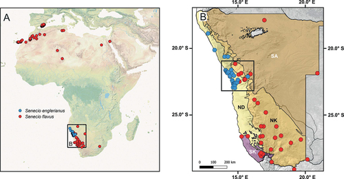
Figure 2. Habitat, phenotypes and pappus hairs of Senecio englerianus and S. flavus. (A) Gravelly coastal habitat of S. englerianus in the hyper-arid Central Namib Desert (near Swakopmund, population 3; see Table 1), associated with fruticose lichens (e.g. Teloschistes capensis) and Pencil Bush (Arthraerua leubnitziae, Amaranthaceae; see also Jürgens et al. 2013). (B) Rocky outcrop habitat of S. flavus in the (semi-)arid Nama-Karoo (near Keetmanshoop, ca. 500 km south of Windhoek); here, the species is known to occur (B. Nordenstam, pers. comm.; see also Figure 1B), but was not found there during field work in April 2005. (C) Individual of S. englerianus near Swakopmund (population 3); the insert shows a large, cushion-forming individual from the same area (population 4) with more than a single year’s growth. (D) Individual of S. flavus from south-western Morocco/Anti-Atlas. (E) Non-fluked (‘typical’) pappus hairs of S. englerianus, with forward-pointing teeth. (F) Connate-fluked pappus hairs of S. flavus, with grappling-hook-like appendages (reproduced from Coleman et al. 2003, with permission from Wiley & Sons, UK, 2 December 2021). Photographs by Joseph J. Milton (A – C), Jean-Paul Peltier (D; CC BY-NC 4.0), and Max Coleman (E,F).

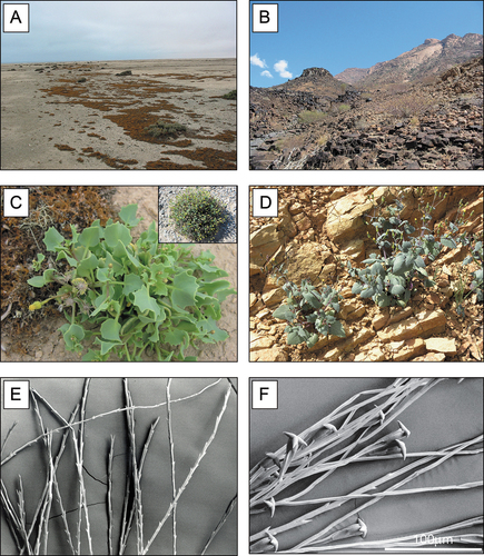
Table 1. Locality information of populations and accessions of Senecio englerianus and S. flavus used for phylogenetic (phyl), morphometric (morph) and experimental-crossing analyses (marked with an asterisk). GenBank accession numbers are provided for all previously published and newly generated ITS sequences (the latter in italics).

Species	Population number/code^a	Country, locality	Latitude	Longitude	Elev (m)	N (phyl)	N (morph)	Collector(s) (herbarium code)	GenBank accession^b
S. englerianus	1	Namibia, Huab River	NA	NA	NA	1	–	Muller & Loutit 1164 (M)	AF457417^S, P
S. englerianus	2 *	Namibia, Swakopmund, road between Walvis Bay and Rooikop Airport, nr. quarry on the D road off the C14 road	22° 40’ S	14° 33’ E	60	1	6	JJM 110.1 (E)	ON924633^P
S. englerianus	3 *	Namibia, Swakopmund, lichen-desert between Swakopmund and Henties Bay, ca. 40 km from Swakopmund	22° 21’ S	14° 26’ E	24	1	7	JJM 111.1 (E)	ON924634^P
S. englerianus	4	Namibia, Swakopmund, Henties Bay, in dried up mouth of Omaruru River	22° 07’ S	14° 17’ E	3	1	–	JJM 113.1 (E)	ON924635^P
S. flavus	MA	Namibia, Maltahöhe	24° 29’ S	16° 58’ E	1,346	1	–	Merxmüller & Giess 28206 (M)	AF457416^S, P
S. flavus	TA (SF) *	Morocco, Souss-Massa Region, Tafraoute, roadside on outskirts of town	29° 43’ N	08° 58’ W	1,000	2	5	AA & RJA s.n. (STA)	TA1: ON924636^P TA2: ON924637^P
S. flavus	AS (SF751) *	Morocco, Marrakesh-Safi Region, 21 km from Asni (near Imgdal)	31° 07’ N	08° 07’ W	1,568	1	–	Ait Lafkih et al. 751 (RNG)	AF457414^S
S. flavus	FU (SF2615)	Spain, Canary Isl., Fuerteventura, Puerto de la Peña/Ajuy	28° 24’ N	14° 09’ W	97	1	1	Nydegger 26145 (RNG)	AF457415^P
S. flavus	SI	Egypt, Sinai, road from Sharm-El Sheik to Dahab	28° 30’ N (approx.)	34° 30’ E (approx.)	0	1	–	Coleman 10/00 (E)	AJ400782^P

Abbreviations: N, number of individuals used for phylogenetic (phyl) and morphometric (morph) analyses, respectively; NA = not available; Elev, elevation (in metres above sea level); collector abbreviations: AA, Anna Abbott; JJM, Joseph J. Milton; RJA, Richard J. Abbott; herbarium abbreviations: E, Royal Botanic Garden Edinburgh Herbarium; M, Munich Herbarium (Botanische Staatssammlung München); RNG, University of Reading Herbarium; STA, University of St Andrews Herbarium.

^aPopulation codes of S. flavus given in parentheses refer to those in Milton (2009).

^bSequences included in the BEAST analysis of Senecioneae (Figure 3 and S1) and ML analysis of the ‘petiolate’ clade of S. englerianus/S. flavus (Figure S2) are indicated by superscripts ‘S’ and ‘P’, respectively.

Figure 3. BEAST-derived maximum clade credibility (MCC) chronogram of Senecioneae, plus one member of Athroismeae (Anisopappus pinnatifidus), based on ITS sequences, with collapsed major clades. Numbers above branches indicate Bayesian posterior probability (PP) values. Branches in dashed lines indicate PP ≤ 0.95. Designation of clades within Senecio s. str. largely follows Kandziora et al. (2017). Mean estimates of stem (A) and crown (B) ages for the ‘petiolate’ clade (in million years ago, Mya) are indicated, together with 95% highest posterior density (HPD) intervals (in parentheses). Respective time estimates and 95% HPDs for all other major clades and single species lineages are summarised in Table S8. Pleis, Pleistocene. See Figure S1 for the full MCC chronogram of all 403 accessions (ca. 363 spp.).

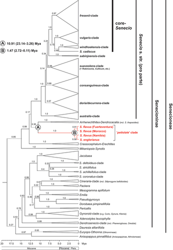
Figure 4. (A) HUMBOLDT-derived principal component analysis (PCA) biplot, along with density plots for each component (PC1, PC2), depicting the extent of environmental niche overlap (purple) between Senecio englerianus (blue) and S. flavus (red) in Southwest Africa. Percentages of total variance explained by each component are shown in parentheses. Filled kernel isopleths represent kernel densities from 1–100%. Empty kernel isopleths represent the 1% density isopleths of the environments (not species) outside boundaries of environmental (E) space. (B) Corresponding correlation circle of 12 bioclimatic variables (see Table S4 for code identification) and elevation (Elev). The length and directionality of arrows (vectors) illustrate, respectively, the strength of contribution (loading) and sign of correlation (positive, negative) of each variable on the two components (PC1: x-axis; PC2: y-axis). Variables closer to each other are thus more correlated on a given component. Analyses were conducted based on 63 locality records (S. englerianus: N = 30; S. flavus: N = 33; see also Figure 1B).

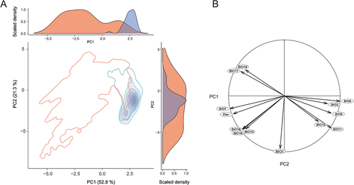
Table 2. Means (± S.E.) of 14 trait variables (C1–C14) measured on 13 individuals of Senecio englerianus (six from population 2, seven from population 3), six individuals of S. flavus [five from Morocco (TA), one from Fuerteventura (FU)] and four F₁ hybrids created by crossing the two species (i.e. two individuals each of crosses AS.1 × 3.29 and TA.5 × 2.2; see text). Shared superscript letters indicate no significant difference at the 5% level using Tukey’s multiple comparisons HSD (honestly significant difference) test. One-way analysis of variance (ANOVA) F-value significance: * P <0.05; ** P ≤0.01; *** P ≤0.001; NS, not significant. Note, non-normally distributed measurements of size (C1–C8) were natural log-transformed, and C14 was arcsine transformed.

Code	Character^a	S. englerianus N = 13	S. flavus N = 6	F1 hybrids N = 4	ANOVA F	F-value significance
C1	Plant height (mm)	165.69 ± 6.38^A	220.83 ± 24.54^B	327.50 ± 24.02^C	26.0	***
C2	Inflorescence length (mm)	20.54 ± 1.28^A	14.83 ± 1.47^B	19.50 ± 1.66^A, B	3.84	*
C3	Peduncle length (mm)	11.23 ± 1.23^A	6.67 ± 1.17^A	11.50 ± 1.66^A	3.06	NS
C4	Capitulum length (mm)	9.31 ± 0.35^A	8.00 ± 0.73^A	8.00 ± 0.00^A	2.78	NS
C5	Capitulum width (mm)	4.46 ± 0.19^A	2.80 ± 0.10^B	5.50 ± 0.29^C	27.6	***
C6	Mean calyculus bract length (mm)	0.77 ± 0.14^A	0.90 ± 0.04^A	1.18 ± 0.06^A	1.65	NS
C7	Longest leaf length (mm)	21.38 ± 1.37^A	41.67 ± 2.01^B	27.75 ± 1.65^A	37.9	***
C8	Midleaf length (mm)	15.46 ± 1.38^A	32.83 ± 2.76^B	21.25 ± 1.80^A	21.9	***
C9	Number of midleaf lobes	9.46 ± 0.63^A	17.83 ± 1.56^B	15.75 ± 0.25^B	24.6	***
C10	Midleaf apical vein angle (°)	45.19 ± 2.30^A	51.00 ± 3.57^A, B	57.50 ± 3.23^B	3.76	*
C11	Midleaf secondary vein angle (°)	39.15 ± 3.00^A	46.50 ± 4.45^A	46.25 ± 3.75^A	1.37	NS
C12	Standardised leaf perimeter (mm)^b	6.38 ± 0.56^A	15.17 ± 0.95^B	5.50 ± 0.50^A	45.7	***
C13	Standardised square root of leaf area (mm^2)^b	1.69 ± 0.24^A	7.33 ± 1.20^B	1.50 ± 0.29^A	27.0	***
C14	Percentage water in midleaf (%)	91.12 ± 0.99^A	79.45 ± 3.76^B	87.48 ± 1.60^A, B	9.17	***

^aSee Table S5 for details of trait measurements, and Table S6 for full data matrix.

^bDivided by the midleaf length.

Figure 5. Principal component analysis (PCA) biplot of 14 quantitative trait variables (C1–C14) measured for Senecio englerianus (N = 13), S. flavus (N = 6; Morocco, Fuerteventura), and F₁ hybrids (N = 4). Percentages of total variance explained by each component (PC1, PC2) are noted in parentheses. Ellipses were fitted to the PCA plane (rather than to the full multivariate data set) so as to include 95% of the points in each of the three groups. See Table 2 for identification of trait codes (C1–C14), and Table S5 for details of trait measurements as well as factor loadings and variable contributions (in %) for each component.

Table 3. Mean estimates of pollen number (grains per floret) and percentage pollen fertility in Senecio englerianus (specimen 3.29), Moroccan S. flavus (AS.1), one of their F₁ hybrids [AS.1 × 3.29 (1)], and 32 individuals of the F₂ generation, produced after self-pollination of this F₁ hybrid. Standard errors are shown in parentheses.

	S. englerianus (3.29)		S. flavus (AS.1)		F1 hybrid		F2 generation
	N = 1	No. of florets	N = 1	No of florets	N = 1	No. of florets	N = 32	No. of florets
Mean pollen number/floret	3394.40 (153.15)	5	495.20 (46.95)	5	409.0 (31.52)	5	1825.35 (48.14)	110
Mean pollen fertility (%)	99.0 (0.23)	10	89.68 (4.36)	10	59.3 (2.00)	5	85.24 (1.20)	110

N refers to the number of individuals. See Table S7 for full data.

Figure 6. (A) Histogram of mean pollen counts for Senecio englerianus × S. flavus F₂ hybrids (N = 32) with fitted normal distribution (solid line), using R. (B) Histogram of mean percentage pollen fertility in the same F₂ generation. Smooth long-dashed and solid lines indicate expected F₂ frequencies according to two normal distributions for the ‘low’ and ‘high’ F₂ series, respectively, as fitted by the R package MIXTOOLS. Note, after curve fitting, one individual from the ‘high’ class (marked by an asterisk) appeared to fall into the ‘low’ class, resulting in an exact ratio of 9 : 7 (see text).

Figure 7. Ecological niche models (ENMs) for Senecio englerianus (A–C) and Southwest African S. flavus (D–G) in Namibia and adjacent regions at the present (1950–2000), the mid-Holocene Climate Optimum (HCO, ca. 6 kyr ago), and the Last Glacial Maximum (LGM, ca. 22 kyr ago). For each time period, potential distributions are also shown at the continental scale (see inserts A–E, and enlarged figure G for S. flavus at the LGM). ENMs were generated in MAXENT on the basis of 11 current bioclimatic variables and a total of 66 specimen records (S. englerianus: N = 30; S. flavus: N = 33; see text for details). Predicted distribution probabilities (ranging from zero to one) are shown in each 2.5 arc-minute pixel. In G, the white-dashed lines delimit the African Dry Corridor (ADC) during arid periods of the Pleistocene according to Neumann and Scott (2018). LVR, Lake Victoria Region. See Figure S3 for corresponding ENMs of S. flavus based on all 150 locality records from across the range of the species.

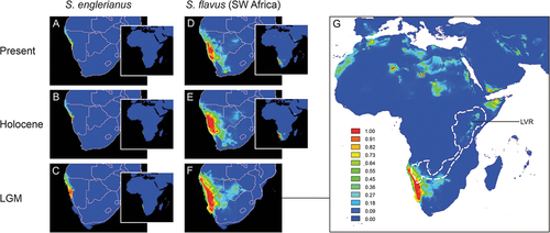
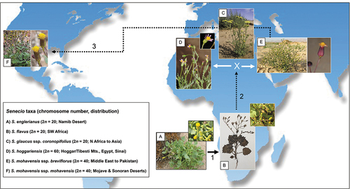
Figure 8. Hypothesised, step-like biogeographic scenario involving (1) the origin of Senecio flavus from S. englerianus in the Namib Desert region, followed by (2) its spread to North Africa (Liston et al. 1989; Coleman et al. 2003; this study), where hybridisation with S. glaucus ssp. coronopifolius gave rise to S. hoggariensis and S. mohavensis ssp. breviflorus, respectively (Kadereit et al. 2006). Note the cross-continental dispersal (3) of the latter taxon to south-western North America (Coleman et al. 2003), followed by the origin of ssp. mohavensis. Photographs by Joseph J. Milton (A: habitus), David Forbes (A: close-up); Richard J. Abbott (B: habitus, collection Bertil Nordenstam), Fouad Msanda (B: close-up; CC BY-NC 4.0), Philippe Geniez (C; BY-NC 4.0), Ori Fragman-Sapir (D; and E: close-up; www.Flora.org.il); Mori Chen (E: habitus; www.Flora.org.il), and Stan Shebs (F; CC BY-SA 4.0). Worldmap (Wagner II projection) by Tobias Jung (CC BY-NC 4.0).

Irish J. 1994. The biomes of Namibia, as determined by objective categorisation. Res Nat Mus, Bloemfontein. 10:549–592.

 Google Scholar

Jürgens N, Oldeland J, Hachfeld B, Erb E, Schultz C. 2013. Ecology and spatial patterns of large-scale vegetation units within the central Namib Desert. J Arid Environ. 93:59–79. doi:10.1016/j.jaridenv.2012.09.009.

 Google Scholar

Coleman M, Liston A, Kadereit JW, Abbott RJ. 2003. Repeat intercontinental dispersal and Pleistocene speciation in disjunct Mediterranean and desert Senecio (Asteraceae). Am J Bot. 90(10):1446–1454. doi:10.3732/ajb.90.10.1446.

 Google Scholar

Milton JJ. 2009. Phylogenetic analyses and taxonomic studies of Senecioninae: Southern African Senecio sect. Senecio [ PhD thesis]. University of St Andrews.

 Google Scholar

Kandziora M, Kadereit JW, Gehrke B. 2017. Dual colonization of the Palaearctic from different regions in the Afrotropics by Senecio. J Biogeogr. 44(1):147–157. doi:10.1111/jbi.12837.

 Google Scholar

Ma T, Wang K, Hu Q, Xia Z, Wan D, Wang Q, Feng J, Jiang D, Ahani H, Abbott RJ, et al. 2018. Ancient polymorphisms and divergence hitchhiking contribute to genomic islands of divergence within a poplar species complex. Proc Natl Acad Sci U S A. 115(2):E236–243. doi:10.1073/pnas.1713288114.

 Google Scholar

Liston A, Rieseberg LH, Elias TS. 1989. Genetic similarity is high between intercontinental disjunct species of Senecio (Asteraceae). Am J Bot. 76(3):383–388. doi:10.1002/j.1537-2197.1989.tb11325.x.

 Google Scholar

Kadereit JW, Uribe-Convers S, Westberg E, Comes HP. 2006. Reciprocal hybridization at different times between Senecio flavus and Senecio glaucus gave rise to two polyploid species in North Africa and South-West Asia. New Phytol. 169(2):431–441. doi:10.1111/j.1469-8137.2005.01604.x.

 Google Scholar

Data availability statement

Data on locality records, voucher specimens (Nordenstam collection) and ITS sequence alignments are available upon request to [email protected]