Figures & data
Figure 1. Overview of the timeline of altimetry missions.
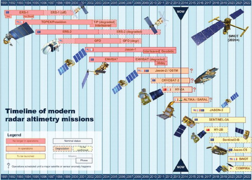
Figure 2. Relative contribution of each altimeter in the multi-mission AVISO/DUACS maps for 2012-2013 and link with altimeter events. The contribution is derived from the degrees of freedom of signal analysis described by CitationDibarboure et al. (2011a). Unit: %.
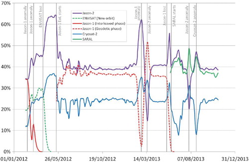
Figure 3. Variance of the pass-band filtered (50-500 km) sea level anomaly from Jason1 and Jason-2 before and after the orbit change of Jason-1 (also known as Extension of Life or geodetic phase). There is a variance increase of the order of 2.5 cm RMS when a gridded mean sea surface is used for the geodetic phase (as opposed to mean tracks for exact repeat orbits).
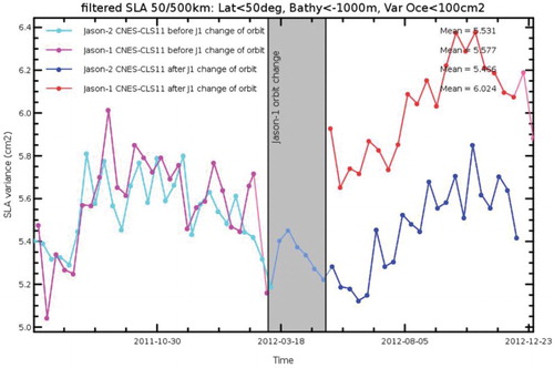
Figure 4. (from CitationMulet et al. 2012): Standard deviation (cm/s) over the global ocean of the differences between zonal and meridonal mean currents from in-situ data and from three MDTs derived from successive releases of GOCE geoids: EGM_TIM_R1 (blue stars), EGM_TIM_R2 (blue diamonds) and EGM_TIM_R3 (blue circles). Black diamonds show the results from the ITG-GRACE-2010s geoid. Black triangles show the standard deviation of the in-situ currents.
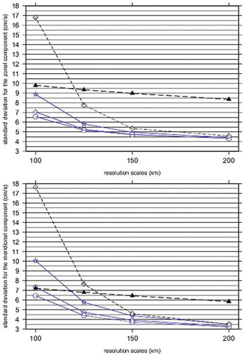
Figure 5. Mean speed (units cm/s) of the geostrophic surface currents for the period 1993-2012 obtained from the combination of altimetry, gravity, hydrographic measurements and drifter data.
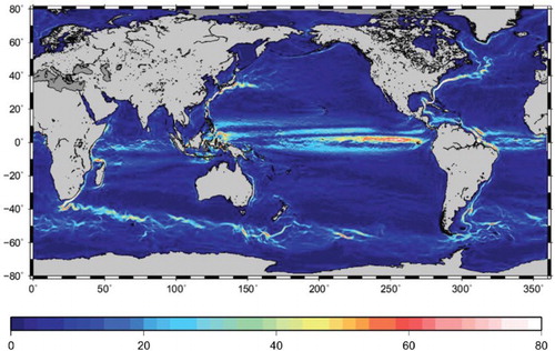
Figure 6. NRT Global, North West Atlantic, Mediterranean, Black Sea regional data distributed by MyOcean Ocean Colour Thematic Assembly Center (OC TAC). L3 daily products (left panels) and corresponding L4 products (right panels). Units are mg/m3.
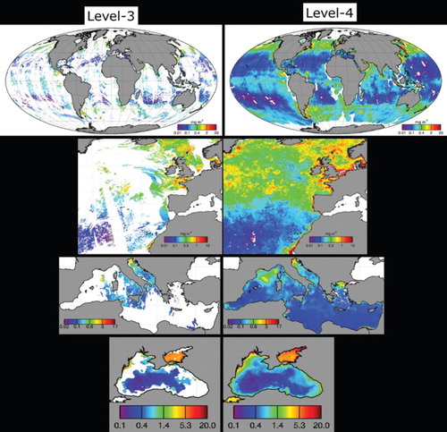
Figure 7. Example of blended wind fields estimated from corrected QuikSCAT and ASCAT wind observations for the four epochs (00h:00, 06h:00, 12h:00, 18h:00 UTC) of February, 2nd 2008 during tropical cyclone Hondo. Circles indicate cyclone path. Units are m/s.
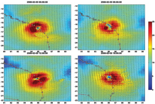
Figure 8. Sea Surface Salinity from SMOS data in the Gulf Stream Region averaged over a 10 day period superimposed with coincident currents from altimetry (left). Monthly global averaged SSS from Aquarius sensor. Units are psu.
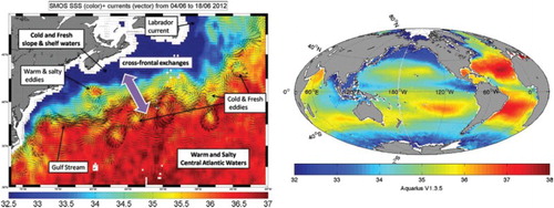
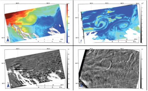
Figure 9. Surface expression of mushroom like eddy structure and filaments with a scale of 5-50 km. (Upper left) MODIS SST map, (lower left) the mean square slope derived from the MODIS reflected shortwave signal, (upper right) MODIS derived chlorophyll-a map, and (lower right) the contemporaneous Envisat ASAR backscatter image (from CitationKudryavtsev et al. 2012).