Seasonal forecasting of winds, waves and currents in the North Pacific

Figures & data

Figure 1. (a) Bathymetry of North Pacific from ETOPO1 at 1° spatial resolution. The black line is the great circle between Singapore and San Diego (transect). (b) Transect monthly climatology (January to December) for 10 m wind speed (green; ERA-Interim); significant wave height (blue; ERA-Interim) and ocean surface current speed (red; ORAP5).

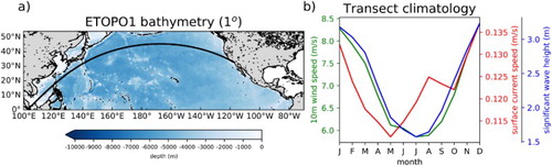
Figure 2. Hovmoller (time-space contour) diagram with (a), (c) and (e) averaged over longitude (100°–290°) and (b), (d) and (f) averaged over latitude (0°–60°). The time axis is given as monthly climatology (January to December). (a) and (b) are 10-m wind speed (ERA-Interim); (c) and (d) are ocean surface current speed (ORAP5); (e) and (f) are significant wave height (ERA-Interim). The average value for the month is given as text above the plots in (a), (c) and (e) and to the right of the plot in (b), (d) and (f).

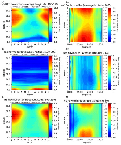
Figure 3. July 10-m wind speed for the period 1993–2013. The panels on the left are the mean 10-m wind speed and the panels on the right are the standard deviation of 10-m wind speed for the respective data sets. (a) and (b) buoy data; (c) and (d) satellite altimeter data (Globwave); (e) and (f) ERA-Interim; and (g) and (h) CCSM4 July forecast using 1st July initial conditions.

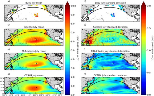
Figure 4. July ocean surface current speed for the period 1993–2013. The panels on the left are the mean ocean surface current speed and the panels on the right are the standard deviation of ocean surface current speed for the respective data-sets. (a) and (b) drifter data; (c) and (d) Satellite altimeter data (Armor-3D); (e) and (f) ORAP5; and (g) and (h) CCSM4 July forecast using 1st July initial conditions.

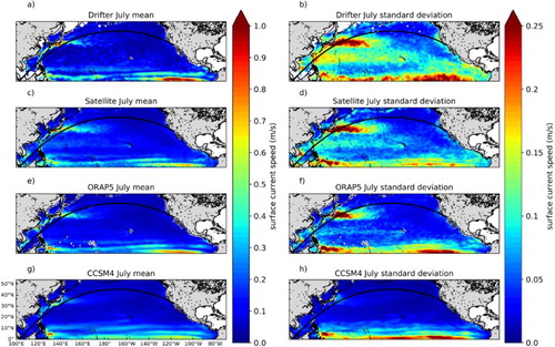
Figure 5. July significant wave height (H_s) for the period 1993–2013. The panels on the left are mean H_s and the panels on the right are standard deviation of H_s. (a) and (b) buoy data; (c) and (d) satellite altimeter data (Globwave); (e) and (f) ERA-Interim; and (g) and (h) CCSM4 forced WAVEWATCH III July forecast using 1st July initial conditions.

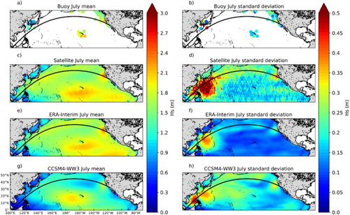
Figure 6. July 90th percentile 1993–2013 for top row: daily 10-m wind speed; middle row: 5-day average ocean surface current speed; bottom row: daily significant wave height. First column: re-analyses (ERA-interim for 10-m wind speed and significant wave height; ORAP5 for ocean surface current speed); second column: CCSM4 July forecasts using 1st July initial conditions;

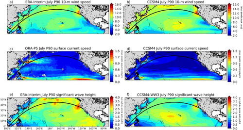
Figure 7. July significant wave height (H_s) averaged over six buoys near Hawaii (51001, 51002, 51003, 51004, 51100 and 51101). Buoy measurements (black), satellite altimeter data (red), ERA-Interim (green) and CCSM4-WW3 July forecast using 1st July initial condition (blue). The 10 ensembles for CCSM4-WW3 are shown as box plots where the extent of the box shows the quartiles and the line is the median value. The whiskers show the extent of the data and the outliers are plotted as filled circles. The July observed values of the Pacific Meridional Model (PMM), El Niño Southern Oscillation (ENSO) and Pacific Decadal Oscillation (PDO) are overlaid as text beneath the plot. In addition, the correlations of the observed H_s with the teleconnection indices are shown in black text in the bottom right.

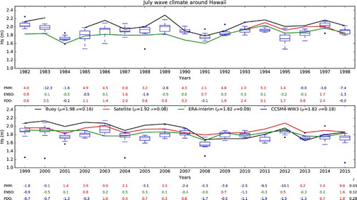
Figure 8. CCSM4 forecast skill of simulating July 10 m wind speed compared to ERA-Interim using 1st July initial conditions. (a) Anomaly correlation; (b) RMSE; (c) Ensemble spread; (d) Saturation RMSE; (e) Rank Probability Skill Score and (f) Normalized Relative Operating Characteristic Area. The stippling on the anomaly correlation shows areas where the correlation coefficient is significantly different from 0 at the 95th percentile level.

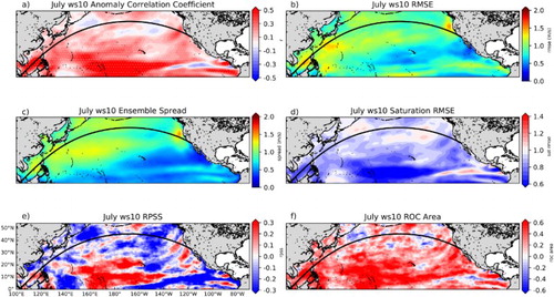
Figure 9. CCSM4 forecast skill of simulating July ocean surface current speed compared to ORAP5 using 1st July initial conditions. (a) Anomaly correlation; (b) RMSE; (c) Ensemble spread; (d) Saturation RMSE; (e) Rank Probability Skill Score and (f) Normalized Relative Operating Characteristic Area.

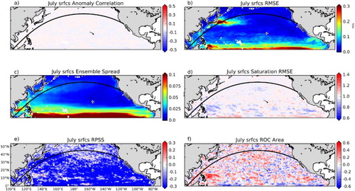
Figure 10. CCSM4-WW3 forecast skill of simulating July significant wave height (H_s) compared to ERA-Interim using 1st July initial conditions. (a) Anomaly correlation; (b) RMSE; (c) Ensemble spread; (d) Saturation RMSE; (e) Rank Probability Skill Score and (f) Normalized Relative Operating Characteristic Area. The stippling on the anomaly correlation shows areas where the correlation coefficient is significantly different from zero at the 95th percentile level.

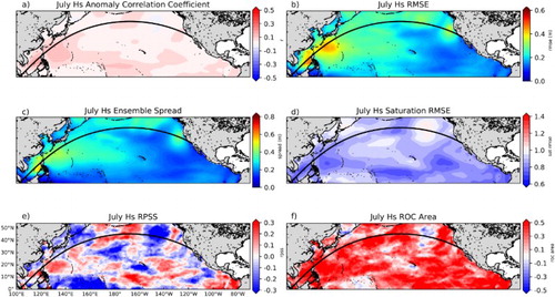
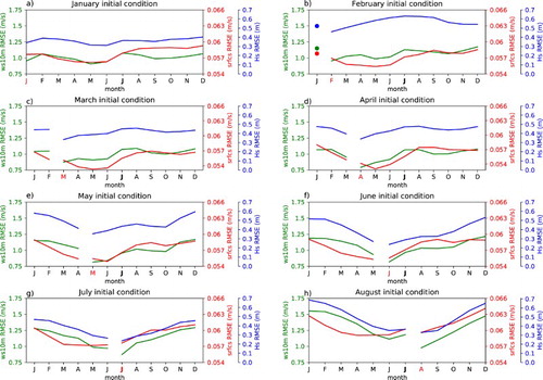
Figure 11. CCSM4 and CCSM4-WW3 RMSE averaged along the transect (Figure 1(a)) for all forecast months using initial conditions 1st January to 1st August. The points which make up the transect are weighted by area as the cosine of the latitude. The x-axis is January to December; the initial condition month is in red and July is always in bold font on the x-axis. The green line is RMSE for 10-m wind speed; the red line RMSE for ocean surface current speed and the blue line RMSE for significant wave height (H_s). Panels (a)–(h) are the initial conditions from January to August.