Figures & data
Figure 1. The data coverage (shaded) during 2010 in percentage (%). The dots show the grid points of the ADC data. The locations of the comparison points at near shore (N; 85.81 E, 19.55 N)) and offshore (O; 86.19 E, 19.17 N) are indicated by the triangle symbol. Black contours denote the isobaths of −50, −200, −500, −1000, −1500 and −2500 m from ETOPO2. Red dots indicate HFR stations at Puri and Gopalpur in the state of Odisha, India. Also shown are the two coastal stations (Paradip and Vizag), where the tide gauge data were collected.
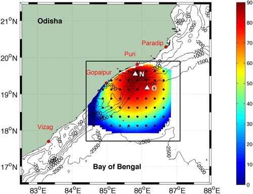
Figure 2. The current direction and magnitude in m/s (Sticks) for (a) HFR in upper panel and (b) ADC in lower panel at location ‘O’ for the year 2010.
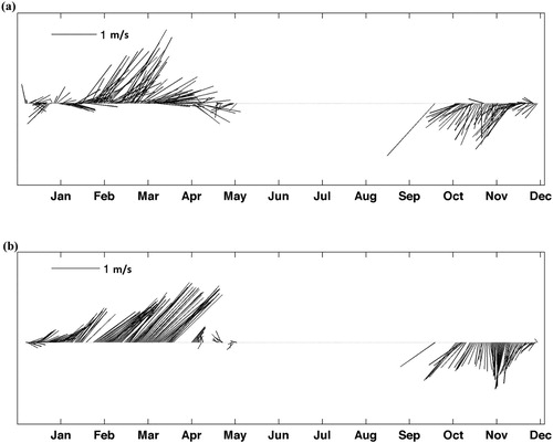
Figure 3. Comparison of daily currents from HFR and ADC (scatter dots) at O location (top), correlation maps (middle) and root mean square error (RMSE) maps (lower) during 2010 for zonal component (left) and meridional component (right). The lines through the regression plots (top panels) indicate the best fit line with value of ‘m’ for its slope and ‘c’ for the intercept. Region-wide Correlation and RMSE (in m/s) (middle and bottom panels) are colour coded to indicate their respective magnitudes. The ‘+’ signs indicate the points with significant level more than 95%.
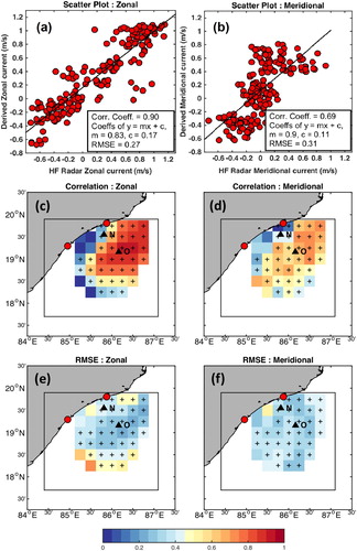
Figure 4. HF radar-derived daily average fields of surface current in m/s (vector) with SSHA in m (shaded) for different months of 2010. Red dots indicate HFR stations at Puri and Gopalpur in the state of Odisha, India. The red line denotes 200 m isobaths.
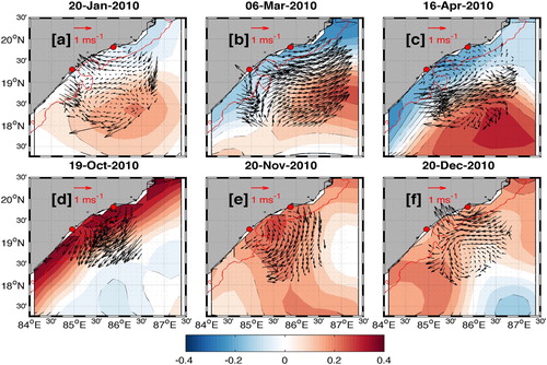
Figure 5. The bars indicate the magnitude of tidally driven current (in cm/s) from HFR current data for 28 constituents at location (a) ‘N’ and (b) ‘O’ for January 2010, derived by using harmonic analysis for u-component (gray) and v-component (black).
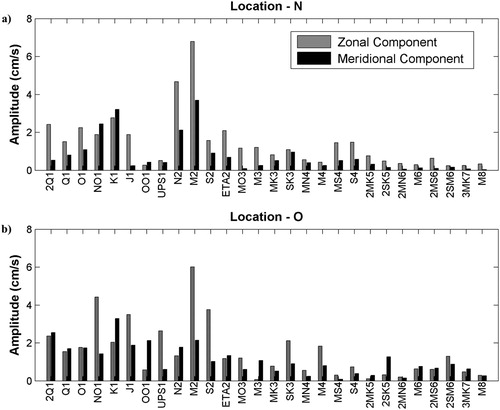
Figure 6. The bars indicate the amplitude of sea level height (in cm) from tide gauge data for 28 constituents at location (a) Paradip and (b) Vizag. Note the correspondence of relative amplitudes of the constituents with those in , indicating the validity of HFR data enabling further high-frequency analysis.
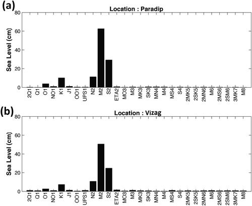
Figure 7. The amplitude of shallow water constituents for tidal-driven current (in cm/s) from HFR data at location (a) ‘N’ and (b) ‘O’; and for sea level (in cm) from tide gauge data at (c) Paradip and (d) Vizag.
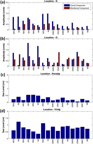
Table 1. Ellipse characteristics from harmonic tidal analysis of currents (u + iv) at the location ‘N’ for January 2010.
Table 2. Ellipse characteristics from harmonic tidal analysis of currents (u + iv) at the location ‘O’ for January 2010.
Figure 8. (a) M2 and (b) MS4 tidal ellipses derived from harmonic analysis of HFR current data. The blue (red) ellipses mean clockwise (counter-clockwise) rotation. The black contours indicate the isobaths. Black ellipse is the reference ellipse. Red dots indicate HFR stations at Puri and Gopalpur, Odisha, India.
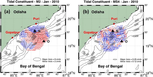
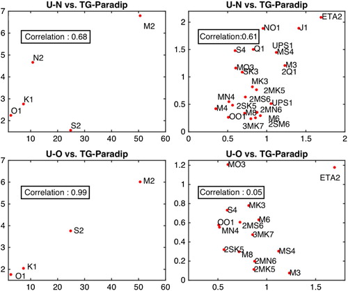
Figure 9. The correlations between the major (left panel) and minor (right panel) tidal constituents (in terms of amplitude) obtained from HFR (y axis in cm/s) derived zonal component at N (top) and O (bottom) locations with tide gauge at Paradip (x axis in cm).