Figures & data
Figure 1. Hs evolution observed for the 6 buoys during the study period (01/12/2013–31/01/2014).
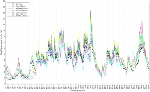
Table 1. Wind datasets characteristics.
Table 2. Buoys location and depth (real and interpolated at the numerical grids).
Figure 2. a) Nesting set-up and computational grids G1, G2 and G3 placements and b) bathymetry of the G2 computational area. The two sectors of the study area are, Atlantic (West) and Cantabrian (North), marked with black intermediate lines and the red isoline indicates the border of the continental shelf. Additionally, the locations of wave buoys are shown with yellow squares.
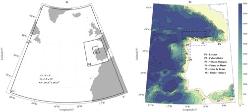
Figure 3. Measured and modelled Hs for the period between 01.12.13–31.01.14. Red dots represent buoys measurement, dotted lines are SWAN results for each wind dataset considered. The bold line indicates the best fit for each buoy. a) Comparison of measurements and G1 computational grid. b) Measured and modelled results with ERA5 wind data, representing all three computational grids in buoy locations P2 and P5.
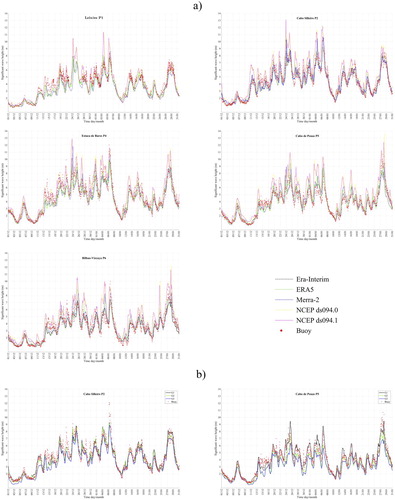
Table 3. RMSE, SI, BIAS and Cor for each computational domain (G1, G2 and G3) at buoys location for a) significant wave height, b) mean wave period and c) wave peak direction. The most optimal dataset for each domain is marked in bold.
Figure 4. Measured and modelled Tm02 for the period between 01.12.13–31.01.14. Red dots represent buoys measurement, dotted lines are SWAN results for each wind dataset considered. The bold line indicates the best fit for each buoy. a) Comparison of measurements and G1 computational grid. b) Measured and modelled results with ERA5 wind data representing all three computational grids, in buoy locations P2 and P5.
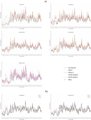
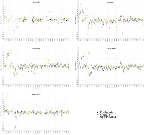
Figure 5. Difference between buoys and model outcome (buoy-SWAN, G1 computational domain) with three wind datasets, ERA-Interim, Merra-2 and NCEP ds094.0.