
Figures & data
Figure 1. Top – Map of the study region with the nominal locations of the observations indicated – dropsonde observations are collected at the same sites as the CTD/LADCP. Contours represent bottom depth from the Smith and Sandwell (Citation1997) data set; solid green indicates land. Note: the global Smith-Sandwell topography data set does not reproduce well the fine details around the Bahama Banks – the eastern pressure gauge is actually at about 13 m depth despite the contours shown in the plot. Bottom – Vertical section of meridional velocity from repeated LADCP observations at the nine stations shown in the top panel. All LADCP sections collected during July 2009 through September 2014 were averaged for this section. Pressure gauge locations are indicated by the black dots. Bottom topography (directly measured) indicated in gray in the lower panel is based on averages from repeat ship sections along the section in the 1980s and 1990s courtesy of Jimmy Larsen.
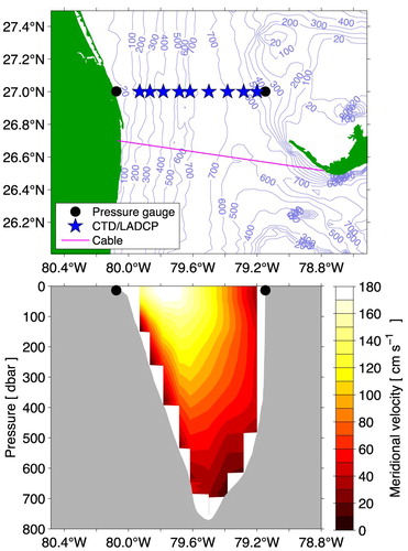
Table 1. Nominal locations of the moored and shipboard observations. The endpoints for the cable are near West Palm Beach (26° 42’N, 80° 04’W) and Eight Mile Rock (26° 31’N, 78° 47’W).
Figure 2. Top: Raw 5-min pressure anomalies from western location. Middle: Raw 5-min pressure anomalies from eastern location. Bottom: Daily average pressure anomalies after a simple 3-day low-pass filtering; note smaller y-axis scale in bottom panel. Vertical black dashed line indicates problematic turn-around discussed in text.
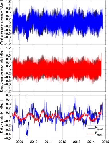
Table 2. Statistics for the six largest-amplitude tidal constituents found through harmonic analysis of the pressure records. Note that the same six constituents were the largest in both pressure records, however the order of amplitude was not the same in the two records. Units: tidal frequencies are in cycles per day; amplitudes are in decibars; phases are in degrees relative to Greenwich. Errors shown for both amplitude and phase are 95% confidence limits. The complete record was used for the east side; for the west side the record beginning on 1 October 2009 was used to avoid the problematic time period discussed in the text where one of the gauges was clogged with debris.
Figure 3. (a) Daily time series of the Florida Current volume transport from the submarine cable (green), the eastern pressure anomaly record minus the western pressure anomaly record (magenta), and the western pressure anomaly record multiplied by −1 (blue). (b) Scatter plot of the daily cable values and the corresponding daily pressure differences. (c) Scatter plot of the daily cable values and the corresponding daily western pressure anomalies multiplied by −1. Angle brackets indicate that all values have been normalized by removing the record-length mean and dividing by the standard deviation of the daily values.
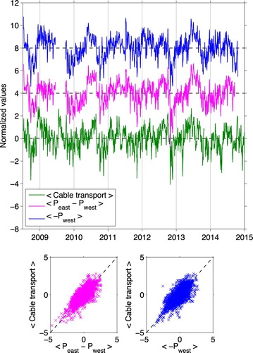
Figure 4. (a) Daily seasonal climatology of the observed pressure records; (b) same but for the pressure difference (east minus west); (c) same but for the cable transports. All climatologies determined as 90-day low-pass filtered records of three-repeated-year climatologies, with only the center year kept to avoid edge effects. Filter was a second order Butterworth, passed both forward and backward to avoid phase shifts.
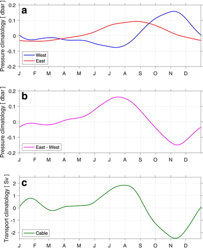
Figure 5. (a) Variance preserving spectra of the daily-averaged west and east pressure records. (b) Variance preserving spectrum of the pressure difference (east minus west). (c) Variance preserving spectrum of the Florida Current volume transport from the cable record during the coincident time period. All spectra were calculated using the Welch’s averaged periodogram method with a two-year window allowing one-year of overlap. Black vertical dashed lines highlight the annual and semi-annual periods. Dashed colored lines indicate the 95% confidence limits for the spectra.
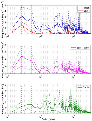
Figure 6. Correlation coefficient r between Florida Current cable transport time series and the pressure difference (Peast – Pwest). Correlation coefficient r is shown for the time series after they have been low-pass filtered with a 2nd order Butterworth filter, passed both forward and backward to avoid phase shifting, with the indicated cut-off periods. Also shown are the 95% and 99% significance levels for the correlation values based on the assumption that the integral time scales of the filtered time series are nominally equal to the filter cut-off period.
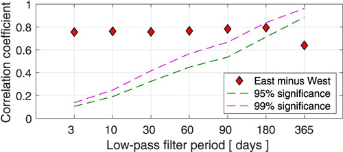
Figure 7. Comparison between direct estimates of Florida Current volume transport from ship sections to estimates of transport from the voltages measured on the cable (red diamonds) and to pressure differences (blue squares), where the pressure differences have been ‘calibrated’ into transport estimates simply by a least-squares fit of the daily pressure differences against the daily cable transports over the full period. Comparisons are shown for the 33 dropsonde sections (a) and the 24 LADCP sections (b) available during the time period overlapping with the pressure gauge data.
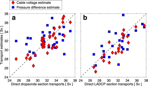
Table 3. Statistics of comparisons between direct measurements of Florida Current volume transport calculated from dropsonde or LADCP ship measurements and the simultaneous transport estimates from the cable or from the pressure differences calibrated into equivalent transport as discussed in the text.
Data availability statement
The pressure/tide gauge data, the LADCP data, and the dropsonde data are available via the Western Boundary Time Series project web page at: www.aoml.noaa.gov/phod/wbts/. The Florida Current cable data are available at www.aoml.noaa.gov/phod/floridacurrent/.