Detection and characterisation of short fatigue cracks by inductive thermography

Figures & data

Table 1. Material parameters

Material	Electrical Conductivity σ [Ω ^−1m^−1]	Relative Permeability µr [-]	Thermal Conductivity λ [W m^−1K^−1]	Density ρ [kg m^−3]	Spec. heat capacity, c [Jkg^−1K^−1]	Penetration Depth δ, if f= 200 kHz [mm]	Thermal Diffusion Length dth, if t= 0.1 s [mm]
Steel ferro-magn.	1.85 × 10^6	600	40	8400	410	0.034	2.16
Steel AISI304 non-magn.	7 × 10^5	1	16	8000	500	1.35	1.26

Figure 1. Gridding around a crack with 1 mm depth and 5 mm length in close-up, by simulating the Joule heating in ferro magnetic steel. a: cross-section through the middle of the crack; at the surface, at the end of the crack and close to the crack line the grid size is strongly reduced. b: Gridding at the surface around the crack tip; high grid density is applied around the crack line and around the crack tip, where a heating hot spot occurs

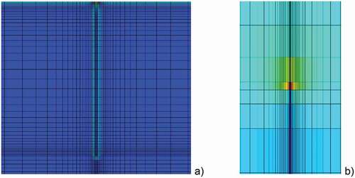
Figure 2. Magnitude of the magnetic field (a, c) around a 10 mm long and 1 mm deep crack; and the temperature distribution after 0.1 s inductive heating pulse with 200 kHz excitation frequency (b, d). Figs. a and b are calculated for ferro-magnetic steel; c and d for austenitic steel. The images show only the half of the model in order to see also the distribution below the surface in the middle of the crack [20]

Figure 3. Temperature distribution after 0.1 s heating around a 10 mm long and 1 mm deep crack in ferro-magnetic steel (a) and in austenitic steel (b); phase images for the same cracks: (c) in ferro-magnetic steel and (d) in austenitic steel; phase images for a short crack with 2 mm length and 1 mm depth in ferro-magnetic steel (e) and in austenitic steel (f) [20]

Figure 4. Phase profiles along the crack calculated for different crack lengths; heating pulse = 0.1 s, crack depth = 1 mm, in ferro-magnetic steel (a), austenitic steel (b). In both figures the line belonging to the shortest crack length, where the phase value in the mid of the crack is approximately equal to the phase value of a very long crack, is plotted as a thick black line

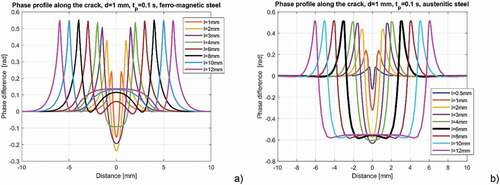
Figure 5. Phase profiles along the crack calculated for different crack depths; heating pulse = 0.1 s, crack length = 10 mm, in ferro-magnetic steel (a), in austenitic steel (b). In figures c and d phase profiles across the cracks in the mid positions are compared to the ones across long cracks, the latter ones are plotted by dashed lines; Figures e and f show the phase plotted as a surface with the definitions for the profiles: red lines mark the phase profile along the crack and yellow lines show for the phase profile across the crack in its middle

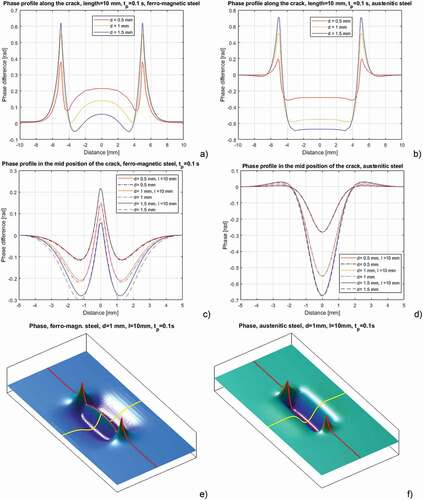
Figure 6. Phase at the crack tip (Φ_max) and phase at the middle of the crack (Φ_min) depending on the length of the crack, calculated for three different crack depth values. For the simulations austenitic steel parameters were used, heating pulse = 0.1 s, excitation frequency = 200 kHz. In the diagram the phase difference to the phase at the sound surface is plotted

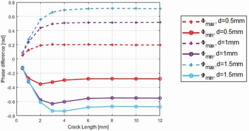
Figure 7. A and b show the two different ways to define the phase contrast for ferro-magnetic steel; c: Φ_max at the crack tip calculated for three different crack depth values and plotted in dependency of the crack length; d: both phase contrasts according to Eqs.5(5) ${\mathrm{\Phi }}_{contrast1}={\mathrm{\Phi }}_{crack}-{\mathrm{\Phi }}_{min}$(5) and 6(6) ${\mathrm{\Phi }}_{contrast2}={\mathrm{\Phi }}_{crack}-{\mathrm{\Phi }}_{sound}$(6) , for the same cracks as in fig.c; the simulations were calculated for heating pulse = 0.1 s and excitation frequency = 200 kHz

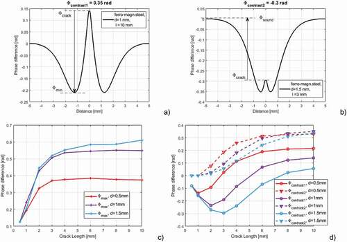
Figure 8. Simulation results for 10 mm long and 1 mm deep vertical cracks in ferro-magnetic steel with different cross-section profiles; top a: rectangular profile, l_depth = 10 mm, bottom a: l_depth = 5 mm, fig. b: comparing the profiles along the crack; fig. c: sketch of the trapezoid shaped crack with the length definitions

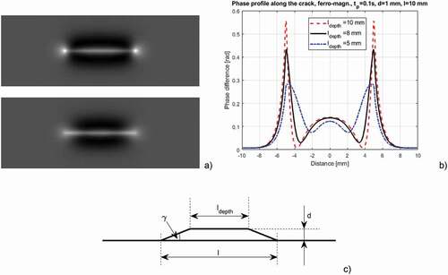
Figure 9. Simulation results for 10 mm long and 1 mm deep vertical cracks in austenitic steel with different cross-section profiles; top a: rectangular profile, l_depth = 10 mm, bottom a: l_depth = 5 mm, fig. b: comparing the profiles along the crack

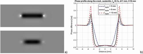
Figure 10. Phase maximum, phase minimum and contrast for ferro-magnetic (a) and for austenitic (b) steel, comparing cracks with rectangular shape (l_depth = l_surf) and cracks with trapezoid shape (l_depth < l_surf)

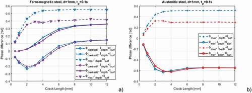
Figure 11. Phase profiles along the crack calculated for different excitation frequencies, crack depth = 1 mm, crack length = 10 mm, in ferro-magnetic steel (a) and in austenitic steel (b)

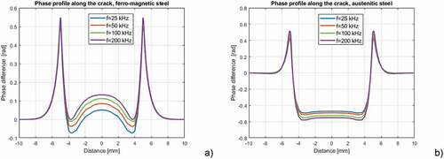
Figure 12. Phase profiles along the crack calculated for different heating pulse durations, crack depth = 1 mm, crack length = 10 mm, in ferro-magnetic steel (a) and in austenitic steel (b); phase profiles across the mid of the crack in ferro-magnetic steel (c) and austenitic steel (d)

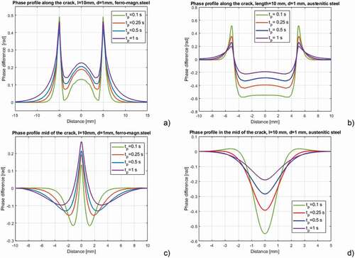
Figure 13. Phase distribution for 1 mm deep and 6 mm long cracks in ferro-magnetic steel with different inclination angles below the surface: 90° (a), 60° (b), 45° (c), 30° (d) between crack and surface. The images show 12 × 12 mm² area around the cracks and all the images have the same scaling, corresponding to the colorbar at the right side

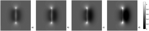
Figure 14. Phase distribution for 1 mm deep and 6 mm long cracks in austenitic steel with different inclination angles below the surface: 90° (a), 60° (b), 45° (c), 30° (d) between crack and surface. The images show 12 × 12 mm² area around the cracks and all the images have the same scaling, corresponding to the colorbar at the right side

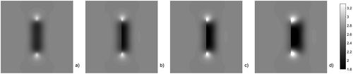
Figure 15. Phase distribution for 1 mm deep and 6 mm long vertical cracks in ferro-magnetic steel with different angles between the crack lines and the induced eddy currents: 90° (a), 60° (b), 45° (c), 30° (d). The images show 12 × 12 mm² area around the cracks and all the images have the same scaling, corresponding to the colorbar at the right side

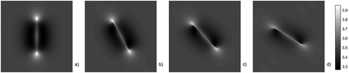
Figure 16. Phase distribution for 1 mm deep and 6 mm long vertical cracks in austenitic steel with different angles between the crack lines and the induced eddy currents: 90° (a), 60° (b), 45° (c), 30° (d). The images show 12 × 12 mm² area around the cracks and all the images have the same scaling, corresponding to the colorbar at the right side

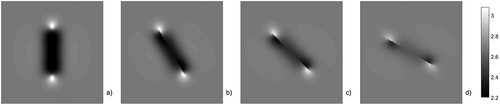
Figure 17. Phase distribution for 1 mm deep and 6 mm long cracks in ferro-magnetic steel, all the cracks have 30° inclination angle to the surface and different angles between the crack lines and the induced eddy currents: 90° (a), 60° (b), 45° (c), 30° (d). The images show 12 × 12 mm² area around the cracks and all the images have the same scaling, corresponding to the colorbar at the right side

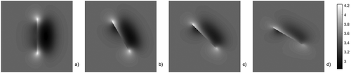
Figure 18. Phase distribution for 1 mm deep and 6 mm long cracks in austenitic steel, all the cracks have 30° inclination angle to the surface and different angles between the crack lines and the induced eddy currents: 90° (a), 60° (b), 45° (c), 30° (d). The images show 12 × 12 mm² area around the cracks and all the images have the same scaling, corresponding to the colorbar at the right side

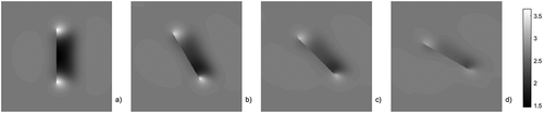
Figure 19. a: Phase image of a 12 mm long crack in ferro-magnetic steel sample after 0.1 s heating pulse duration; b: phase image of a 6 mm long fatigue crack in austenitic steel after 0.5 s heating pulse duration [19,20]

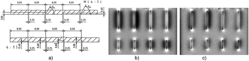
Figure 20. A: CAD drawing of the sample with artificial cracks; phase images after 0.3 s heating pulse, the induced eddy currents are perpendicular to the crack lines (b) and enclose 45° (c)

Oswald-Tranta B, Tuschl C. Detection of short fatigue cracks by inductive thermography, in Proc. of 15th QIRT Conf., 2020

 Google Scholar

Oswald-Tranta B, Feistkorn S, Rössler G, et al. Comparison of different inspection techniques for fatigue cracks. in Proc. SPIE 11409, Thermosense: Thermal Infrared Applications XLII, 2020

 Google Scholar

Data Availability Statement

The infrared measurement files which were evaluated to obtain Figure 19a, Figure 20b and 20c are openly available at https://zenodo.org/record/5037199