Jaccard matrix for nonlinear filter statistics

Figures & data

Table 1. $2\times 2$ contingency table.

Effect \ Cause	C	$\mathrm{\neg }C$
E	a	c
$\mathrm{\neg }E$	b	d

Table 2. $n\times m$ contingency table.

	$X_0$	···	$X_j$	···	$X_{m-1}$
$Y_0$			$c_{0j}$
⋮			⋮
$Y_i$	$c_{i0}$	···	$c_{ij}$	···	$c_{im-1}$
⋮			⋮
$Y_{n-1}$			$c_{n-1j}$

Figure 1. A sketch of the two-dimensional rectangular space $S^x\times S^y\subset {\mathbb{R}}^2$ to define the Jaccard matrix and the cruciform region $S_1\cup S_2$ to calculate the Jaccard cell.

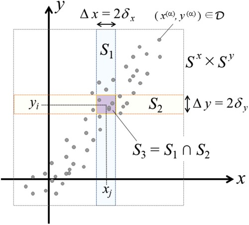
Figure 2. The solid lines of (i) and (ii) show sketches of the graphs of the simple model of the Jaccard cell, Equation (43(43) $\phi =\frac{{\delta }_0}{\text{β}-{\delta }_0}(0<{\delta }_0\le \text{β}/2).$(43) ), in the cases where β or ${\delta }_0$ is fixed as each constant value.

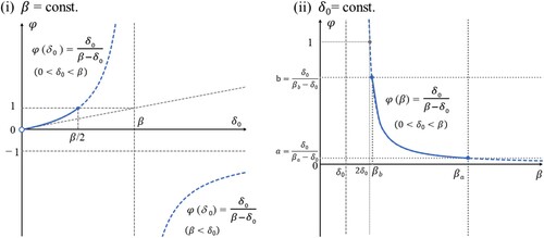
Figure 3. The graphs of the Jaccard cells (JC) based on Equation (33(33) $\left(\mathrm{A}\mathrm{J}\mathrm{C}\right):\psi ({\mu }_x,{\mu }_y;\delta ,\delta )\approx \frac{\delta }{\sqrt{2\pi (1-{\rho }^2)}-\delta }.$(33) ) in $\delta =0.2,0.4,0.6,0.8$, the approximation by (35(35) $\begin{array}{rl}& \left(\mathrm{J}\mathrm{C}\mathrm{M}\mathrm{I}\right):\psi ({\mu }_x,{\mu }_y;\delta ,\delta )\approx \frac{\delta }{\sqrt{2\pi (1-{\rho }^2)}}\\ & =\frac{\delta }{\sqrt{2\pi }}{\mathrm{e}}^{I(X,Y)}.\end{array}$(35) ) in $\delta =0.2,0.4,0.6$, the MI (34(34) $I(X,Y)=-\frac{1}{2}\ln (1-{\rho }^2)=\ln \frac{1}{\sqrt{1-{\rho }^2}}.$(34) ), and the absolute value of the correlation coefficient $|\rho |$.

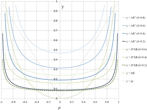
Table 3. The instances of the function to generate test data.

Cos7x	$f\left(x\right)=\cos 7x$, $x\in [0,\pi ]$
Cos14x	$f\left(x\right)=\cos 14x$, $x\in [0,\pi ]$
Sin28x	$f\left(x\right)=\sin 28x$, $x\in [0,1]$
SinVaryingFreq	$f\left(x\right)=\sin \left\{7\pi x\right(x+1\left)\right\}$, $x\in [0,1]$
Parabola	$f\left(x\right)=x^2$, $x\in [-0.5,0.5]$
Cubic	$f\left(x\right)=x^3+x^2-4x$, $x\in [-1.3,1.1]$

Figure 4. The typical behaviour of $\mathrm{A}\mathrm{v}\mathrm{e}\left(\mathrm{\Psi }\right)$, $\mathrm{V}\left(\mathrm{\Psi }\right)$, and $\mathrm{S}\mathrm{D}\left(\mathrm{\Psi }\right)$ for n which defines $n\times n$ Jaccard matrix. These lines are generated by Equation (52(52) $x=u\mathrm{a}\mathrm{n}\mathrm{d}y=f\left(x\right)+r,$(52) ) using the function Cos14x in Table 3 and ${\sigma }_r={10}^{-3}$.

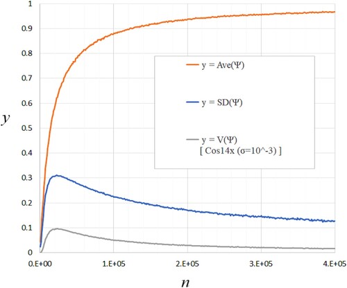
Figure 5. The numerical tests for the theoretical model (46(46) $\begin{array}{rl}& =V\left[\phi \right]\left(\overline{\phi }\right)=-{(\overline{\phi }-\frac{Z_V}{2Z_E})}^2+\frac{Z_V^2}{4Z_E^2}\end{array}$(46) ) expressing the estimation of the relationship between the mean and the variance of the Jaccard cells. The plotted dots are generated by the function Cos14x of ${\sigma }_r={10}^{-3},{10}^{-2},{10}^{-1},{10}^{-0.1}$. The grey dashed line shows the parabolic function $\mathrm{V}\left(\mathrm{\Psi }\right)=-{\alpha }_0\left(\mathrm{A}\mathrm{v}\mathrm{e}\right(\mathrm{\Psi })-{\alpha }_1{)}^2+{\alpha }_2$, where ${\alpha }_0=0.6$, ${\alpha }_1=0.61$, and ${\alpha }_2=0.096$, to approximate the dots of ${\sigma }_r={10}^{-3}$ phenomenologically.

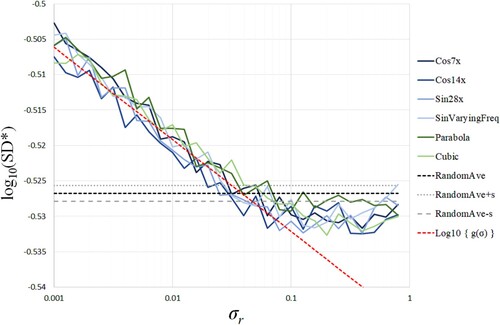
Figure 6. The values of ${\log }_{10}{\mathrm{S}\mathrm{D}}^{\ast }$ for the standard deviation ${\sigma }_r$ of the additional noise r of Equation (52(52) $x=u\mathrm{a}\mathrm{n}\mathrm{d}y=f\left(x\right)+r,$(52) ). The horizontal axis is a logarithmic one for the value of ${\sigma }_r$, and the vertical axis is a normal one for the value of ${\log }_{10}{\mathrm{S}\mathrm{D}}^{\ast }$.