Strong-Form Frequentist Testing In Communication Science: Principles, Opportunities, And Challenges

Figures & data

Figure 1. Three T-distributions.

The shaded area under the curves of the two non-central distributions represents statistical power for a null hypothesis test with $\alpha =.025$ given population effect sizes $\delta =0.3$ and $\delta =0.5$.

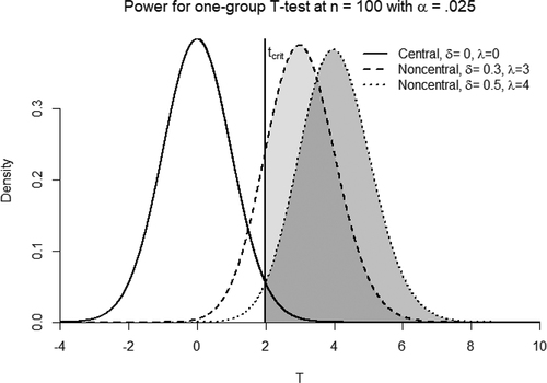
Figure 2. Sampling distribution of $T$-statistics given population effect sizes $\delta =d_{min}$$.\dot{P}$ is represented by the shaded area. The arrows show the direction and strength of corroborators and falsifiers.

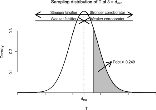
Table 1. Information needed to calculate $\dot{P}$ in R for General Linear Models with fixed effects.

Distribution Family	Type of hypothesis test	Test statistic	Degrees of freedom	Hypothesized (minimal) effect size of interest dmin	Noncentrality Parameter	Function forġ
Z	Sample mean against constant, known variance.	$z=\sqrt{n}\frac{\left(\bar{y}-\mu \right)}{\sigma }$	/	Unstandardized:$\hat{\mathrm{\Delta }}=\left(\bar{y}-\mu \right)$Standardized: $Cohen{ }^{\mathrm{\prime }}s\hat{d}=\frac{\hat{\mathrm{\Delta }}}{\sigma }$	$\lambda =\sqrt{n}\frac{\hat{\mathrm{\Delta }}}{\sigma }$ $=\sqrt{n}\hat{d}$	$\lambda >0:$1 – pnorm (x = z, mean = $\lambda ,$$\mathrm{s}\mathrm{d}=1)$$\lambda <0:$ pnorm (x = z, mean = $\lambda ,$$\mathrm{s}\mathrm{d}=1)$
	Difference of 2 independent sample means, known and equal variances.	$z=\sqrt{\frac{n_1{n}_2}{n_1+n_2}}\frac{\left({\bar{y}}_1-{\bar{y}}_2\right)}{\sigma }$	/	Unstandardized:$\hat{\mathrm{\Delta }}=\left({\bar{y}}_1-{\bar{y}}_2\right)$Standardized: $Cohen{ }^{\mathrm{\prime }}s\hat{d}=\frac{\hat{\mathrm{\Delta }}}{\sigma }$	$\lambda =\sqrt{\frac{n_1{n}_2}{n_1+n_2}}\frac{\hat{\mathrm{\Delta }}}{\sigma }$ $=\sqrt{\frac{n_1{n}_2}{n_1+n_2}}\hat{d}$
T	Sample mean against constant, unknown variance	$t=\sqrt{n}\frac{\left(\bar{y}-\mu \right)}{s}$	$v=n-1$	Unstandardized: $\hat{\mathrm{\Delta }}=\left(\bar{y}-\mu \right)$ Standardized: $Cohen{ }^{\mathrm{\prime }}s\hat{d}=\frac{\hat{\mathrm{\Delta }}}{\sigma }$	$\lambda =\sqrt{n}\frac{\hat{\mathrm{\Delta }}}{\sigma }$$=\sqrt{n}\hat{d}$	$\lambda >0:$ 1 – pt (q = t, df = v, ncp = λ) $\lambda <0:$ pt (q = t, df = $v$, ncp = $\lambda )$
	Difference of 2 dependent (paired) sample means. (“dependent t-test”)	$t=\sqrt{n}\frac{\left({\bar{y}}_1-{\bar{y}}_2\right)}{s_{\left({\bar{y}}_1-{\bar{y}}_2\right)}}$	$v=n-1$	Unstandardized: $\hat{\mathrm{\Delta }}=\left({\bar{y}}_1-{\bar{y}}_2\right)$Standardized: ^1 $\hat{d}=\frac{\hat{\mathrm{\Delta }}}{\sqrt{{\sigma }_1^2+{\sigma }_2^2-2{\rho }_{12}{\sigma }_1{\sigma }_2}}$	$\lambda =\sqrt{n}\frac{\hat{\mathrm{\Delta }}}{{\sigma }_{diff}}$ $=\sqrt{n}\hat{d}$
	Difference of 2 independent sample means, unknown variances. Equal population variances assumed. (“t-test”)	$t=\sqrt{\frac{n_1{n}_2}{n_1+n_2}}\frac{\left({\bar{y}}_1-{\bar{y}}_2\right)}{s}$	$v=n-2$	Unstandardized: $\hat{\mathrm{\Delta }}=\left({\bar{y}}_1-{\bar{y}}_2\right)$ Standardized: $Cohen{ }^{\mathrm{\prime }}s\hat{d}=\frac{\hat{\mathrm{\Delta }}}{\sigma }$	$\lambda =\sqrt{\frac{n_1{n}_2}{n_1+n_2}}\hspace{0.17em}\frac{\hat{\mathrm{\Delta }}}{\sigma }$ $=\sqrt{\frac{n_1{n}_2}{n_1+n_2}}\hat{d}$
T	Difference of 2 independent sample means, unknown variances. Equal population variances not assumed. (“Welch’s t-test”)	$t=\frac{{\bar{y}}_1-{\bar{y}}_2}{\sqrt{(s_1^2/n_1+s_2^2/n_2)}}$	$v\approx \hspace{0.17em}\frac{(s_1^2/n_1+s_2^2/n_2{)}^2}{s_1^4/(n_1^2\left(n_1-1\right)+s_2^4/n_2^2\left(n_2-1\right))}$	Unstandardized: $\hat{\mathrm{\Delta }}=\left({\bar{y}}_1-{\bar{y}}_2\right)$	$\lambda =\frac{\sqrt{n_1{n}_2}}{\sqrt{{\sigma }_1^2{n}_2+{\sigma }_2^2{n}_1}}\hat{\mathrm{\Delta }}$	$\lambda >0:$ 1 – pt (q = t, df = $v$, ncp = λ) $\lambda <0:$ pt (q = t, df = $v$, ncp = $\lambda )$
	Correlation coefficient	$t=\frac{r_{xy}\sqrt{n-2}}{\sqrt{1-r_{xy}^2}}$	$v=n-2$	${\hat{r}}_{xy}$${\hat{r}}_{xy}^2$	$\lambda =\frac{{\hat{r}}_{xy}\sqrt{n}}{\sqrt{1-{\hat{r}}_{xy}^2}}$
	Regression Coefficient (1 independent variable)	$t=\sqrt{n-2}\frac{b_1\sqrt{{\sum }_{i=1}^n{\left(x_i-\bar{x}\right)}^2}}{\sqrt{{\sum }_{i=1}^n{\left(y_i-\widehat{y_i}\right)}^2}}$	$v=n-2$	Unstandardized: ${\hat{b}}_1$ Standardized: $\widehat{{\beta }_1}={\hat{r}}_{xy}$ ${\hat{r}}_{xy}^2$	$\lambda =\widehat{b_1}\sqrt{\frac{n{\sigma }_x^2}{{\sigma }_{\epsilon }^2}}$ $=\frac{{\hat{r}}_{xy}\sqrt{n}}{\sqrt{1-{\hat{r}}_{xy}^2}}$
${\chi }^2$	Independence of 2 categorical variables in a contingency table with k cells. All observations are independent. Decent sample size.	${\chi }^2={\sum }_{j=1}^k{\frac{\left(O_j-E_j\right)}{E_j}}^2$	$v=\left(r-1\right)\left(c-1\right)$	$Cohen{ }^{\mathrm{\prime }}s\hspace{0.17em}\hat{w}$ $=\sqrt{{\sum }_{j=1}^k\frac{{\left({\hat{p}}_{Aj}-{\hat{p}}_{0j}\right)}^2}{{\hat{p}}_{0j}}}$	$\lambda =$ n${\hat{w}}^2$	1 – pchisq (q = X^2, df = $v$, ncp = $\lambda )$
F	Multiple linear regression (Full Model)	$F=\frac{S{S}_m}{S{S}_e}\frac{v_2}{v_1}$	$v_1=p$$v_2=n-1-p$, where p is the number of predictors	${\hat{f}}^2=\hspace{0.17em}\frac{{\hat{R}}^2}{\left(1-{\hat{R}}^2\right)}$	$\lambda =n{\hat{f}}^2$	1 – pf (q = F, df1 = $v_1$, df2 = $v_2$, ncp = $\lambda )$
	Multiple linear regression (Specific predictors)	$F=\frac{R_{change}^2}{\left(1-R_{Total}^2\right)}\frac{v_2}{v_1}$Where $1-R_{Total}^2$ is the unexplained variance in the full model	$v_1=p_{test}$$v_2=n-1-p_{total}$where $p_{total}$ is the total number of predictors, $p_{test}$ is the number of tested predictors	${\hat{f}}^2=\frac{{\hat{R}}_{change}^2}{\left(1-{\hat{R}}_{Total}^2\right)}$Where ${\hat{R}}_{change}^2$ change is the change in explained variance after adding tested predictors	$\lambda =n{\hat{f}}^2$
	Differences of more than 2 independent sample means (“One-Way ANOVA”). Equal variances assumed.	$F=\frac{S{S}_m}{S{S}_e}\frac{v_2}{v_1}$	$v_1=k-1$$v_2=n-k$where k is the number of independent groups	${\hat{f}}^2=\frac{{\hat{\eta }}^2}{\left(1-{\hat{\eta }}^2\right)}$	$\lambda =\sum _{j=1}^k{n}_j{\left(\frac{{\hat{\mu }}_j-{\hat{\mu }}_{grand}}{{\sigma }_{within}}\right)}^2$ $=n{\hat{f}}^2$
	Difference of more than 2 dependent sample means (“repeated measures ANOVA”). Sphericity assumed.	$F=\frac{S{S}_m}{S{S}_e}\frac{v_2}{v_1}$	$v_1=k-1$$v_2=k\left(n-1\right)-n+1$where k is the number of (repeated) groups and n is the number of participants (in each group)	${\hat{f}}^2=\frac{{\hat{\eta }}^2}{\left(1-{\hat{\eta }}^2\right)}$	$\lambda =\frac{nk}{\left(1-\bar{\rho }\right)}{\hat{f}}^2$, where $\bar{\rho }$ is the average correlation in scores between the groups

Note. Except for the Welch $T$-test the formulas reported here have been restricted to cases where $\lambda$ can be straightforwardly expressed as a function of a common (standardized) effect size. See the Technical Appendix for more details. Formulas are also reported in Liu (2014), Cohen (1988), the G*Power manual, and the manual for (2020) software. Suggestive rules-of-thumb for the size of standardized effects $r$, $R^2$, $d$, $w$, and ${\eta }^2$ are mentioned by Cohen (1992, p. 157).

¹$d$ in the paired-samples-formula corresponds to $d$ as calculated by G*Power, with the standardizer in the denominator reflecting the standard deviation of the difference. It has been noted that the standard deviation of the difference is not very easy to interpret substantively, and it is sometimes recommended to use the standard deviation of the baseline to make $d$ more interpretable (Cumming, 2013). However, the formulation as given in this table most easily translates into $\lambda$, which serves the purpose of the current paper.

Figure 3. Distributions of $\delta =0$ and $\delta =d_{min}$ belonging to examples 1, 2, and 3.

The curves illustrate the position of the observed test statistic within the alternative and null distributions, the extent to which it provides corroborating/falsifying information, and the overlap between null and alternative distributions.

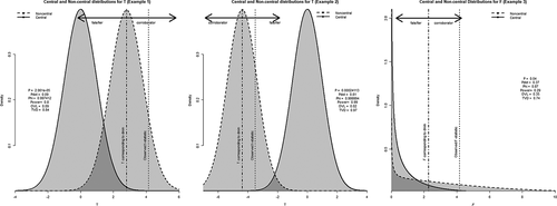
Figure 4. Graph representing the relationship between power, $\phi$ (“falsifiability”), the overlapping coefficient, and the total variation distance.

This graph clarifies that $\phi$ is very high even at low levels of statistical power, which implies that, in general, there is a small probability of corroborating $\delta \ge d{ }_{min}$ if $\delta =0$.

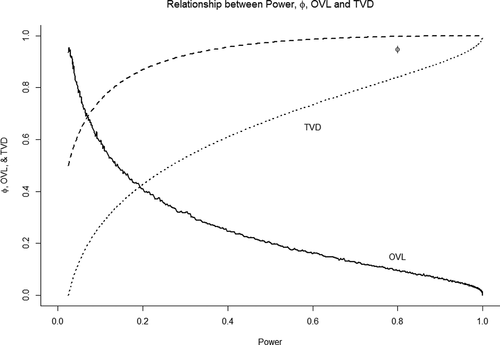
Figure 5. Severity curves for the three examples.

Dots represent values at which $\dot{P}=.05$ and $\dot{P}=.95$.

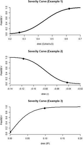
Figure 6. Analytical and simulated pdf’s for $T$.

This graph shows that the simulated probability density function of $T$ overlaps with the analytical solution.

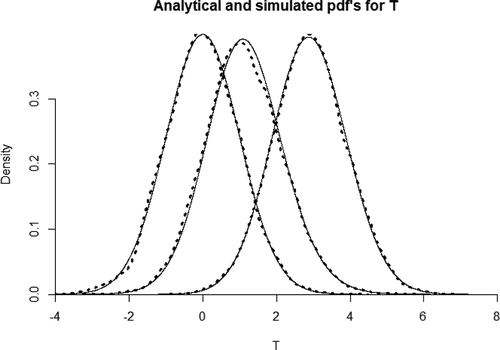
Figure 7. The sampling distribution of $P$ under varying population effect sizes and sample sizes (upper figure), and the sampling distribution of $\dot{P}$ under varying population effect sizes and sample sizes (lower figure).

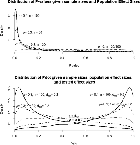
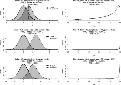
Figure 8. The effects of $\delta =d_{min}$ and sample size (left column) on (1) the overlap between central and non-central distributions (left and middle column), and (2) the distribution of $\dot{P}$ if the null hypothesis is true (right column).

Liu, X. S. (2014). Statistical power analysis for the social and behavioral sciences: Basic and advanced techniques. Routledge.

 Google Scholar

Cohen, J. (1988). Statistical Power Analysis for the Behavioral Sciences. Hillsdale, NJ: Erlbaum.

 Google Scholar

PASS. (2020). Power analysis and sample size software [Computer Software]. NCSS, LLC. ncss.com/software/pass

 Google Scholar

Cohen, J. (1992). A power primer. Psychological Bulletin, 112(1), 155. https://doi.org/10.1037/0033-2909.112.1.155

 PubMed Web of Science ®Google Scholar

Cumming, G. (2013). Cohen’s d needs to be readily interpretable: Comment on Shieh (2013). Behavior Research Methods, 45(4), 968–971. https://doi.org/10.3758/s13428-013-0392-4

 PubMed Web of Science ®Google Scholar