Dsg2 ectodomain organization increases throughout desmosome assembly

Figures & data

Figure 1. Measuring Dsg2 ectodomain order using excitation-resolved fluorescence polarization microscopy. (A) stylized schematic of a desmosome with either ordered (left) or disordered (right) cadherin ectodomains. (B) hypothesized pathways leading to the mature, ordered state of Dsg2 ectodomains (black star): constant (red line), gradual (magenta line), and stepwise (cyan line). (C) the construct used to measure Dsg2 ectodomain order, Dsg2-ECTO. (D) Western blot probing for Dsg2 in WT A-431 cells (left) and A-431 cells stably expressing Dsg2-ECTO (A-431-S, right) with a GAPDH loading control. (E) widefield fluorescence images of A-431 cells stably expressing Dsg2-ECTO (left) and immunolabeled for desmoplakin (DP, middle), with a merged image shown to the right. (F) excitation-resolved fluorescence polarization microscopy of Dsg2-ECTO in A-431-S cells. From left to right: the average intensity across all excitation polarizations with a representative cell border highlighted by a white, rectangular ROI, magnified ROIs showing the emission intensity at each excitation polarization, the azimuth (Az.) directions for each desmosome, and the order Factor (OF). All scale bars represent 10 μm.

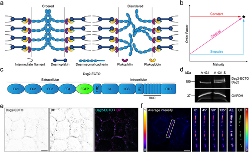
Figure 2. Dsg2-ECTO localizes to desmosomes without impacting the gain of adhesive strength. (A) Representative widefield fluorescence images of A-431-S cells stably expressing Dsg2-ECTO (top row) and immunolabeled for desmoplakin (DP, middle row) during the calcium-free pulse assembly assay. Merged images are shown in the bottom row. Top labels indicate the corresponding assembly time points. Scale bar represents 20 μm. (B) Representative images of A-431-S cells during a dispase fragmentation assay performed after the calcium-free pulse assembly assay. Image labels indicate the corresponding assembly time points. (C) quantification and statistical comparison of the number of fragments at each time point. Error bars indicate mean ± SD for data pooled across three independent experiments, each comprising three technical replicates per time point (n = 9; 2 h: 88.1 ± 24.5; 4 h: 57.7 ± 17.6; 6 h: 41.1 ± 31.8; 8 h: 25.8 ± 14.1; no-pulse: 8.8 ± 6.6). Plot markers corresponding to replicates from independent experiments are each shown as different shapes. Statistical significance was assessed with an ordinary one-way ANOVA followed by Sidak’s multiple comparisons test (****p < 0.0001; *p < 0.05; ns, p ≥ 0.05).

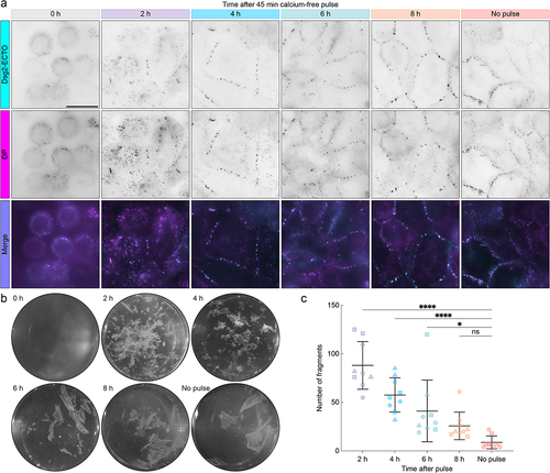
Figure 3. Dsg2 ectodomain order increases gradually during desmosome assembly. (A) normalized average intensity (top) and order factor (OF, middle) images of A-431-S cells acquired 2, 4, 6, or 8 h after a 45 min calcium-free pulse along with the no-pulse control. White rectangles indicate ROIs, which are shown magnified below their corresponding images. An additional set of ROIs is shown to illustrate the pixel azimuth directions (white lines) for each desmosome, where the length of each azimuth line is proportional to the of in its pixel. Scale bars represent 20 μm and 2 μm for full images and ROIs, respectively. (B) swarm plots showing the average of for each desmosome (object OF) across all experiments. Error bars represent median and interquartile range (IQR) (2 h: 0.22, IQR: 0.16–0.31, n = 1020; 4 h: 0.26, IQR: 0.18–0.33, n = 1813; 6 h: 0.30, IQR: 0.22–0.37, n = 1470; 8 h: 0.31, IQR: 0.23–0.38, n = 1258; no-pulse: 0.32, IQR: 0.24–0.39, n = 1108). (C) bar chart showing the circular standard deviation of the azimuth for each desmosome across all experiments. Error bars represent median and IQR (2 h: 12.49, IQR: 6.80–22.99, n = 1020; 4 h: 10.15, IQR: 6.07–17.96, n = 1813; 6 h: 9.08, IQR: 5.68–15.55, n = 1470; 8 h: 7.92, IQR: 4.83–12.65, n = 1258; no-pulse: 7.45, IQR: 4.50–13.02, n = 1108). For both B and C, statistical significance was assessed with a Kruskal–Wallis test followed by Dunn’s multiple comparisons test (****p < 0.0001; **p < 0.01; ns: not significant, p ≥ 0.05).

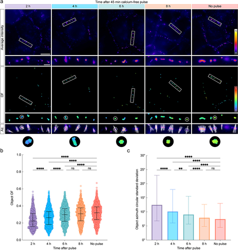
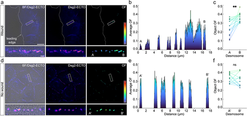
Figure 4. Dsg2 ectodomain order increases gradually along cell borders between migrating cells. (A) from left to right, brightfield (BF) with overlaid average intensity, average intensity, and order factor (OF) of A-431-S cells fixed 2 h after a scratch wound. The leading edge is labeled with a dashed white line. A representative cell border between leading edge cells is highlighted by a white rectangle and shown magnified beneath the corresponding images. Desmosomes closest to and farthest from the leading edge are labeled in the of ROI as ‘A’ and ‘B’, respectively. Scale bars represent 20 μm and 2 μm for full images and ROIs, respectively. (B) two-dimensional line scan between the desmosomes labeled in A, showing the change in average OF along the cell border. (C) paired dot plot showing the difference in OF between desmosomes closest to (‘A’) and farthest from (‘B’) the leading edge for multiple cell borders (means ± SD for n = 15 cell borders: A: 0.26 ± 0.09; B: 0.36 ± 0.05). Statistical significance was assessed with a paired t-test (**p < 0.01). (D-F) same as in A-C for cell borders on the same coverslip but located in fully confluent regions in the cell sheet, far from the leading edge. For each cell border analyzed, A′ and B′ represent desmosomes flanking the border, as depicted in the of ROI in D (means ± SD for n = 12 cell borders: Aʹ: 0.34 ± 0.05; Bʹ: 0.32 ± 0.07). Statistical significance was assessed with a paired t-test (ns: not significant, p ≥ 0.05).

Data availability statement

The data that support the findings in this manuscript are available from the corresponding author, ALM, upon reasonable request.