A Recipe for Disappointment: Policy, Effect Size, and the Winner’s Curse

Figures & data

Figure 1. Contour density plot of the joint distribution of valuations and bids for a simulated auction. The right panel shows densities of bids given a valuation of $13. The top panel shows densities of valuations given a bid of $13. The simulation illustrates bidders whose individual valuations $v\sim \mathcal{N}\left(10,2\right)$ with bid risks $\sim \mathcal{U}\left(v-1,v+1\right).$

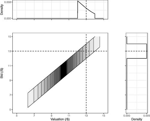
Figure 2. The contour plot of the joint density of $\delta$ and $d$ for a set of simulated studies. The right panel shows a density plot for $p(d|\delta =.6);$ the top panel for $p(\delta |d=.6),$ with the black area illustrating the probability that the estimate and latent effect size have opposite signs. This simulates a large set of studies with underlying latent effect sizes $\delta \sim \mathcal{N}(0,.5)$ and each study estimate $d\sim \mathcal{N}(\delta ,.25).$

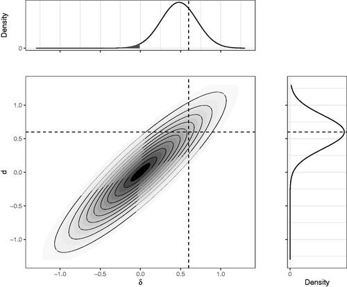
Figure 3. Histogram of symmetrized observed $z$ scores for studies in the EEF set with the fitted mixture model (solid black line) and its two components (dashed).

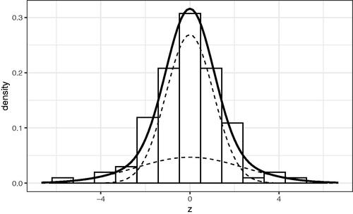
Table 1. Components of models of distribution of $z$ and $\zeta .$

	Proportions	z	$\zeta$
Component 1	0.28	2.40	2.19
Component 2	0.72	1.06	0.37

Figure 4. Median, 25th, and 75th percentiles of the distribution of the exaggeration ratio $\frac{\left|z\right|}{\left|\zeta \right|}$ conditional on $z.$

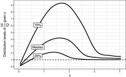
Figure 5. Mean signal-to-noise ratio and probability of exaggeration, given z.

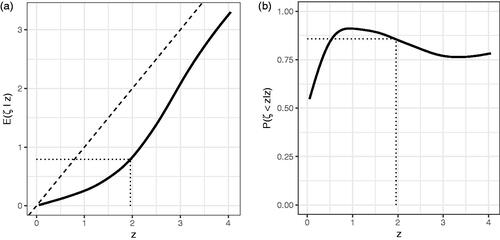
Figure 6. The probability that the latent effect is in the opposite direction conditional on $z.$

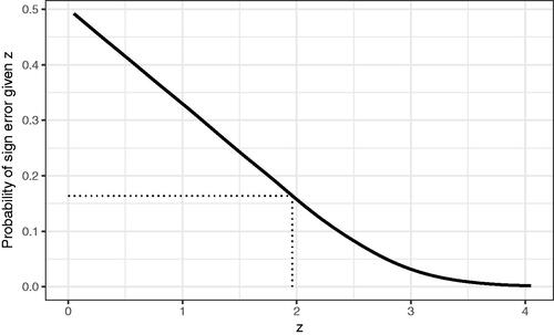
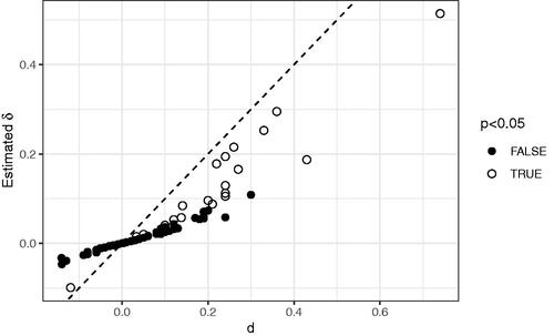
Figure 7. Comparison of predicted power and estimated actual power.

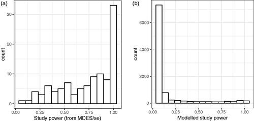
Figure 8. Effect sizes in the set of EEF studies, against their adjusted size.