Design of multi-tier multi-time horizon closed-loop supply chain network with sustainability under uncertain environment for Indian paper industry

Figures & data

Figure 1. Schematic of the proposed CLSC network

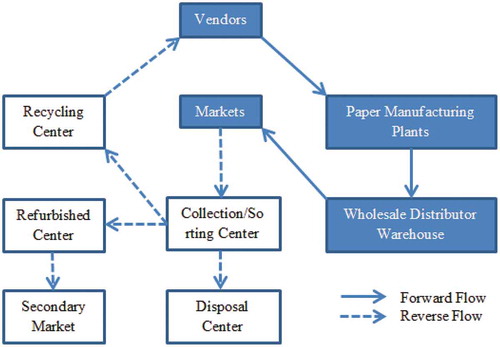
Table 1. Notations used in mathematical model formulations

Notation	Description
H,h	Denotes the number of vendors (h = 1 … …, H)
I,i	Denotes the number of paper manufacturing plant (i = 1 … …, I)
J,j	Denotes the number of wholesale distributor/warehouse (j = 1 … …, J)
K,k	Denotes the number of markets (i.e. customer) (h = k … …, K)
L,l	Denotes the number of collection/sorting centre (l = 1 … …, L)
R,r	Denotes the number of refurbshed centre (r = 1 … …, R)
F,f	Denotes the number of recycling centre (f = 1 … …, F)
T,t	Denotes the number of secondary market (t = 1 … …, T)
Z,z	Denotes the number of the disposal site (z = 1 … …, Z)
B	Denotes the number of raw material, (b = 1,2 …., B)
v	Unit selling price of per ton of paper
u	Unit quantity revenue generated through recycling
w	Unit selling price of per ton of paper in secondary market
Vhe	Set of vehicle at node h in period e, h є H, denoted by vh, vh = 1,2 … … vh
Vie	Set of vehicle at node i in period e, I є I, denoted by vi, vi = 1,2 … … vi
Vje	Set of vehicle at node j in period e, j є J, denoted by vj, vj = 1,2 … … vj
Vke	Set of vehicle at node k in period e, k є K, denoted by vk, vk = 1,2 … … vk
Vle	Set of vehicle at node l in period e, l є L, denoted by vl, vl = 1,2 … … vl
Vre	Set of vehicle at node r in period e, r є R, denoted by vr, vr = 1,2 … … vr
Vte	Set of vehicle at node t in period e, t є T, denoted by vt, vt = 1,2 … … vt
Vfe	Set of vehicle at node f in period e, f є F, denoted by vf, vf = 1,2 … … vf
Vze	Set of vehicle at node z in period e, z є Z, denoted by vz, vz = 1,2 … … vz
Fie	Fixed cost of manufacturing plant in period e
Fje	Fixed cost of wholesale distributor warehouses in period e
Fle	Fixed cost of collection centre in period e
Fre	Fixed cost of refurbished centre in period e
Ffe	Fixed cost of recycling centre in period e
Fze	Fixed cost of disposal site in period e
Chie	Unit ton shipping cost from vendor source h to plant i in period e
Cije	Unit ton shipping cost from paper manufacturing plant i to wholesale distributor warehouse j in period e
Cjke	Unit ton shipping cost from wholesale distributor warehouse j to market k in period e
Ckle	Unit ton shipping cost from market k to collection/sorting centre l in period e
Clre	Unit ton shipping cost from collection centre l to refurbished centre r in period e
Crte	Unit ton shipping cost from refurbished centre r to secondary market t in period e
Clfe	Unit ton shipping cost from collection centre l to recycling centres f in period e
Clze	Unit ton shipping cost from collection centre l to disposal site z in period e
Cfhe	Unit ton shipping cost from recycling centre f to vendor h in period e
$v_{me}$	Tons of demand quantity in period e
$C_{bhie}$	Unit ton cost of raw material in period e
$C_{phie}$	Unit ton cost of production in period e

Table 2. Decision variables

Notations	Descriptions
xhie	Quantity to be sent from vendor h to manufacturing plant i in period e
xije	Quantity to be sent from manufacturing plant i to wholesale distributor warehouse j in period e
xjke	Quantity to be sent from wholesale distributor warehouse j to market k in period e
xkle	Quantity to be sent from market, i.e. customer to collection/sorting centre in period e
xlre	Quantity to be sent from sorting/collection centre l to refurbished centre r in period e
xrte	Quantity to be sent from refurbished centre r to the secondary market t in period e
xlfe	Quantity to be sent from sorting/collection centre l to recycling centre f in period e
xlze	Quantity to be sent from sorting/collection centre f to disposal site z in period e
xfhe	Quantity to be sent from recycling centre f to vendor in period e
xzze	Received quantity (in ton) at disposal site in period e
$x_{bhie}$	Ton of raw material quantity flow in period e
$x_{phie}$	Ton of quantity of unit produced in period e
$N_{vhe}$	No. of truck vh hired by hth vendor in period e
$N_{vie}$	No. of truck vi hired by ith manufacturing plant in period e
$N_{vje}$	No. of truck vj hired by jth wholesale distributor warehouses in period e
$N_{vke}$	No. of truck vk hired by kth market in period e
$N_{vle}$	No. of truck vl hired by lth collection centre in period e
$N_{vre}$	No. of truck vr hired by rth refurbished centre in period e
$N_{vte}$	No. of truck vt hired by tth secondary market in period e
$N_{vfe}$	No. of truck vf hired by fth recycling centre in period e
$N_{vze}$	No. of truck vz hired by zth disposal site in period e
Yie	1 if paper manufacturing plant is established at site i, 0 otherwise in period e
Yje	1 if wholesale distributor warehouse is established at site j, 0 otherwise in period e
Yle	1 if collection centre is established at site l, 0 otherwise in period e
Yre	1 if refurbished centre is established at site r, 0 otherwise in period e
Yfe	1 if recycling centre is established at site f, 0 otherwise in period e
Yze	1 if disposal site is established at site z, 0 otherwise
Sh	Capacity of vendor hth in tons
Ki	Potential capacity of plant at site i in tons
Wj	Potential warehouse capacity at site j in tons
Ll	Potential capacity of collection/sorting centre at site l in tons
Ff	Potential capacity of recycling centre at site f in tons
Rr	Potential capacity of refurbished centre at site r in tons
Zz	Potential capacity of disposal site z in tons
βme	Rate of utilisation of mth item in period e
${\mu }_{be}^m$	Rate of return of mth item in period e by market k
γme	Rate of refurbished of mth item in period e
ηbe	Ratio of recycling for bth material per unit of mth item in period e
Cap	Capacity avaialble for each truck

Table 3. Various parameters of the given problem

Each vendor’s raw material capacity	2000 ton
Capacity of production for each plant	1250 ton
Each wholesale distributor warehouse storage capacity	1000 ton
Each collection/sorting centre capacity	750 ton
Each refurbished centre capacity	350 ton
Each recycling centre capacity	500 ton
Each disposal site capacity	400 ton
Capacity of each trucks	10 ton
Rate of conversion	0.75
Ratio of return	0.7
Ratio of refurbished	0.20 to 0.30 of product (in ton) at collection/sorting centre
Ratio of disposal	0.10 to 0.25 of product (in ton) at collection/sorting centre
Ratio of recycling	0.60 to 0.75 of product (in ton) at collection/sorting centre

Table 4. Unit ton (raw material + transportation) cost (in million Rs. (₹)) from vendor to manufacturing plants

Vendor\manufacturing plant	I1	I2	I3
H1	12	14	17
H2	14	15	15
H3	13	15	12
H4	12	14	11

Table 5. Unit ton (production + transportation) cost (in million Rs. (₹)) for raw material sent to wholesale distributor warehouse

Paper manufacturing plant/wholesale distributor warehouse	J1	J2	J3	J4	FC
I1	4	4	6	12	3750
I2	3	5	3	4	3500
I3	3	7	4	6	3500

Table 6. Unit ton associated transportation cost (in million Rs. (₹)) from whole distributor warehouse (J) to market (K) & fixed cost (in million Rs. (₹)) of warehouses along with demand for all three periods

Wholesale distributor/market	K1	K2	K3	K4	K5	K6	FC
J1	2	2	3	4	4.5	2.5	1400
J2	1	4	4.5	5	3.5	2	1350
J3	2	3	4	6	1.5	4	1400
J4	1.5	2.5	3	3	2	2	1500
D_1 (in ton)	200	140	160	200	500	400
D_2 (in ton)	220	160	180	220	540	420
D_3 (in ton)	240	180	200	240	580	480

Table 7. Unit ton associated transportation cost (in million Rs. (₹)) from market (K) to collection/sorting centre (L)

Market/collection centre	L1	L2	L3
K1	0.8	1	0.8
K2	0.6	0.33	0.6
K3	1	1	1
K4	1	1.2	1
K5	0.5	0.5	0.5
K6	0.33	0.45	0.33

Table 8. Unit ton associated transportation cost (in million Rs. (₹)) from collection/sorting centre (L) to refurbished centre (R) & fixed cost (in million Rs. (₹)) of collection/sorting centre

Collection centre/refurbished centre	R1	R2	FC
L1	0.2	0.5	1150
L2	0.4	0.3	1000
L3	0.1	0.6	1150

Table 9. Unit ton associated transportation cost (in million Rs. (₹)) from refurbished centre (R) to secondary market (T) & fixed cost (in million Rs. (₹)) of refurbished centre

Refurbished centre/secondary market	T1	T2	T3	T4	T5	T6	FC
R1	2	1	2	1	3	2	750
R2	1	1	2	0.5	3	2.5	800

Table 10. Unit ton (in million Rs. (₹)) associated transportation cost from collection/sorting centre (L) to recycling centre (F)

Collection centre/recycling centre	F1	F2
L1	0.3	0.5
L2	0.25	0.6
L3	0.4	0.5

Table 11. Unit ton associated transportation cost (in million Rs. (₹)) from collection centre (L) to disposal site (Z) & fixed cost (in million Rs. (₹)) of disposal sites

Collection centre\disposal site	Z1	Z2
L1	0.32	0.5
L2	0.4	0.8
L3	0.1	0.25
FC	750	750

Table 12. Unit ton associated transportation cost (in million Rs. (₹)) from recycling centre (F) to vendor (H)

Recycling centre\vendors	H1	H2	H3	H4	FC
F1	0.4	0.3	0.3	0.25	1000
F2	0.2	0.6	0.6	0.2	1000

Table 13. Scenario of case 1 for different periods

Time period	Supply chain cost (in million Rs. (₹))	No. of trucks required	Revenue generated (in million Rs. (₹))	SC surplus, i.e. profit (in million Rs. (₹))
1	47,167.66	390	63,780	16,612.34
2	47,978.91	399	73,506	25,527.09
3	52,399.44	445	81,522	29,122.56

Figure 2. Optimal product flow and network configuration between echelons in forward supply chain for case 1

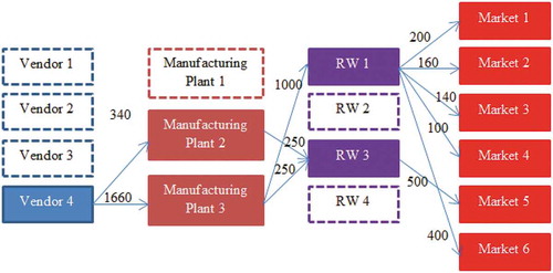
Figure 3. Optimal product flow and network configuration between echelons in reverse supply chain for case 1

Table 14. Scenario of case 2 for different periods

Time period	Supply chain cost (in million Rs. (₹))	No. of trucks required	Revenue generated (in million Rs. (₹))	SC surplus, i.e profit (in million Rs. (₹))
1	47,413.3	386	65,900	16,486.7
2	48,483.97	396	73,668	25,184.03
3	52,924.07	442	81,384	28,459.93

Table 15. Comparison of existing FSC, case 1 and case 2

	SC surplus, i.e. profit (in million Rs. (₹))			% Improvement of case 1 and 2 over FSC		No. of trucks
Time period	Existing_FSC	CLSC_Case1	CLSC_Case2	A*	B*	Existing_FSC	CLSC_Case1	CLSC_Case2
1	15,435.17	16,612.34	16,486.7	7.09	6.38	302	390	386
2	17,590	25,527.09	25,184.03	31.09	30.15	310	399	396
3	19,820	29,122.56	28,459.93	31.94	30.35	322	445	442

A* – % improvement of case 1 over FSC; B* – % improvement of case 2 over FSC.

Figure 4. Optimal product flow and network configuration between echelons in forward supply chain for case 2

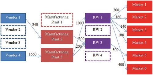
Figure 5. Optimal product flow and network configuration between echelons in reverse supply chain for case 2

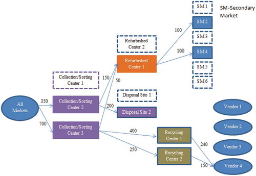
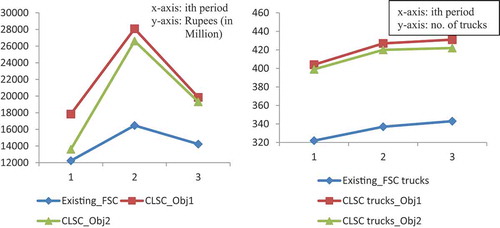
Figure 6. Comparison of SC surplus and number of trucks for existing FSC and proposed CLSC (cases 1 and 2)

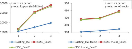
Table 16. Scenario of case 3 for different periods

	Supply chain cost (in million Rs. (₹))		No. of trucks required		Revenue generated (in millions Rs. (₹))		SC surplus, i.e. profit (in million Rs. (₹))
Time period	Prioritising first objective	Prioritising second objective	Prioritising first objective	Prioritising second objective	Prioritising first objective	Prioritising second objective	Prioritising first objective	Prioritising second objective
1	48,151.04	48,734.18	404	399	65,990	62,205.5	17,838.96	13,608.32
2	50,150.04	50,950.08	427	420	78,244	77,568	28,093.96	26,617.92
3	51,041.02	51,417.17	431	422	71,012	70,732	19,850.98	19,314.83

Figure 7. Optimal product flow and network configuration between echelons in forward supply chain for case 3

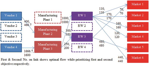
Figure 8. Optimal product flow and network configuration between echelons in reverse supply chain for case 3

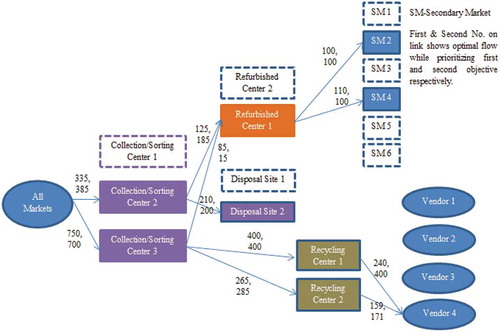
Figure 9. Comparison of SC surplus and no. of trucks for existing FSC and CLSC under uncertain environment for case 3