Figures & data
Figure 1. Geometry of RHT between differential surfaces leading to the definition of differential view factors.
Figure 2. Choice of coordinate system for the computation of P2A view factors and projection of a distant surface Aj onto the HC. Summation of the point-to-pixel view factors belonging to the shaded pixels gives the P2A view factor of Aj. The projection of all distant surfaces Aj is done by rendering them with OpenGL on the graphics card. The camera is located at p and points into the z-direction.
Figure 3. Quadrature subdivision for the computation of obstructed A2A view factors. Details see text.
Figure 4. (Colour online) Pipelining and parallelization of the HC rendering and the summation of the P2Tx view factors. The HC gets rendered into a framebuffer object (FBO), step (0), while the content of another FBO is copied into a pixel buffer object (PBO), step (1). At the same time data from another PBO is copied from the GPU to the CPU side of the PCI-express bus by means of a direct memory access transfer, step (2). Parallel to these buffer operations the contents of a CPU-side copy of a PBO are summed up to get the P2A view factors, step (3). The image in the FBO is a sample image of a rendered HC. Each stage of the pipeline has its own set of FBO, PBO and CPU-side PBO mirror. The tiles in the latter indicate how different parts of the image of the HC are distributed among several threads for computing the P2A from the P2Tx view factors.
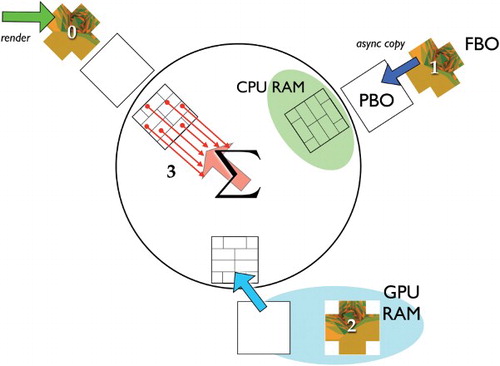
Table 1. Barycentric coordinates (px, py, pz) and weights wα of the 3-point Gauss–Legendre quadrature on a triangle.
Table 2. Computers used in tests.
Figure 5. (a) Geometry of the concentric cubes. Dimensions are 1 m×1 m×1 m and 3 m×3 m×3 m, respectively. Face numbering is such that the sum of the indexes of opposite faces equals 7. For the inner cube we use roman numbers. (b)Mutually different A2A view factors for this scene. The view factors (F1→II and FII→1) are obstructed.
Figure 6. (a) Mesh of the EN442-compliant test cabin. The room is of size 4 m×4 m×3 m. Some elements of the wall supporting the radiator have been removed for view the inside. The radiator consists of only one section. The particular difficulty of this setup is the thin metal sheets attached to the radiator (see the inset). The radiator is 0.6 m high. The single segment is 0.066 m wide and 0.09 m deep. The three-dimensional structure of the convection fins of 0.5 mm thickness is fully resolved. (b)–(d) Distribution of absolute errors in weighted column sums for Ntx=1024, Gauss7, ns=3. On most of the surface elements, the error is in the range from 1e−5 to 1e−3. The outliers are located on only a few pathological elements. (d) The two surface elements with an error of about 30% are the red ones where the convection fin is attached to the body of the radiator segment. On all other surface elements the error is at most 10% and of it is of the order of.01–.1%.
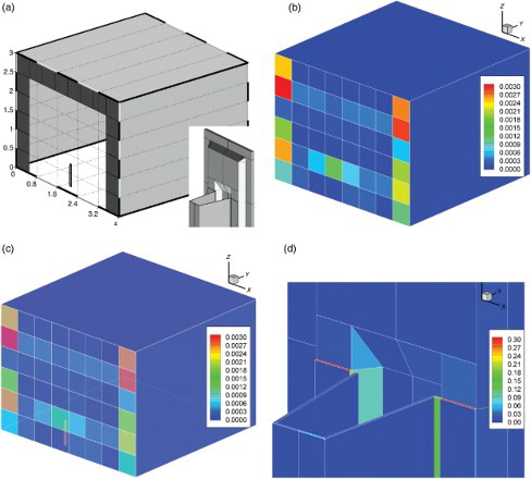
Figure 7. (a) Surface mesh of the warehouse. Some of the elements have been removed for view of the inside. The details of the geometry of the ceramic infrared heaters are shown on the lower left. For further details see text. (b), (c) Distribution of errors in weighted column sums. On most of the surface elements the error is in the range from 1e−5 to 1e−3. The outliers are located on only a few elements which all feature singularities of the view factor kernel at some of their boundaries. Note the logarithmic scale bars. Surprisingly, the weighted column sums on the infrared heaters converge well, (b) Gauss3, Ntx=1024, ns=3 and (c) Gauss3, Ntx=1024, ns=7.
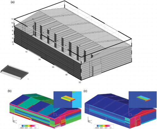
Figure 8. Relative errors of the A2A view factors for the unit cube. The view factor between opposing faces is Fops and Fadj is the one for surface elements sharing an edge. For reasons of symmetry there are only two mutually different view factors. In all cases the best absolute errors were of the order of 10−6. The legend of sub-figure (b) applies to all. (a) Fadj, exact value: 0.200044 and (b) Fops, exact value: 0.199825.
Figure 9. Relative errors of the A2A view factors for the concentric cubes as used in Francisco et al. (Citation2013) (cf. (a)). Our results are several orders of magnitude more accurate than those given in Francisco et al. (Citation2013, Table 5 and ). In all cases the best absolute errors were of the order of 10−6. The legend of sub-figure (a) applies to all. (a) F1→I, exact value: 0.079704; (b) F1→II, exact value: 0.007852; (c) FI→1, exact value: 0.717336; and (d) FII→1, exact value: 0.070666.
Figure 10. Effect of a mismatch between the HC grid and the edge of the projection of a surface element onto the HC. Details see text.
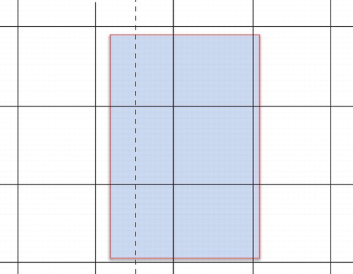
Figure 11. Top: Total CPU times vs. HC dimension for computing the A2A view factor matrix of the concentric cubes (cf. (a)). Bottom: Deviation from unity of the largest and the smallest column sum of the A2A view factor matrix. The column sums are computed from Equation (13). The legend in the top figure applies to all sub-figures.
Figure 12. Deviation from unity of the weighted column sums in case of the warehouse computed on c3, cf. (a) and . We plot the extrema as function of the HC dimension Ntx and the level of quadrature subdivision ns.
Figure 13. Achieved PCIe transfer rates for the warehouse (cf. (a)).
Table 3. Barycentric coordinates (px, py, pz) and weights wα of the 7-point Gauss–Legendre quadrature on a triangle.
Figure 14. Top: Total CPU times vs. HC dimension for the computation of the A2A view factor matrix of the unit cube. Bottom: Deviation from unity of the largest and the smallest column sum of the A2A view factor matrix. The column sums are computed from Equation (13). The legend in the top figure applies to all sub-figures.
Figure 15. Dependence of the total run time on the HC dimension and quadrature subdivision for the warehouse on c3 (cf. (a) and ). For coarse-grained HCs the run time is roughly constant since the overhead in the PCIe transfer dominates. PCIe transfer rates start to saturate for HC dimensions larger than 256.
Figure 16. Relative error of the radiant flux balance for the warehouse (cf. (a)).
Figure 17. Relative error of the radiant flux balance for the test cabin with radiator section (cf. (a)). Despite an error of at least 30% in the weighted column sums (cf. Equation (13)), the radiant flux balance is violated only by about 4%.