Characterization of an airflow network model by sensitivity analysis: parameter screening, fixing, prioritizing and mapping

Figures & data

Figure 1. Twin House O5 – ground floor plan (in colour online).

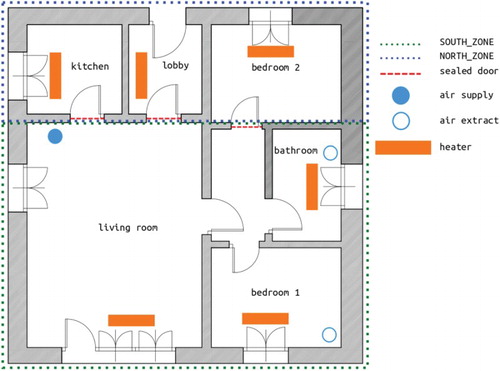
Figure 2. Twin House O5 – flow network model (in colour online).

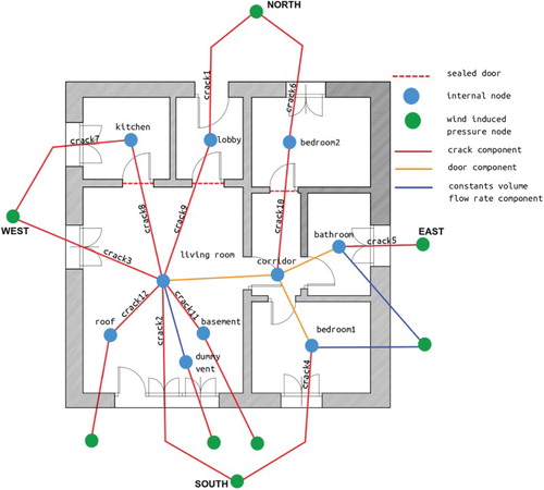
Figure 3. Wind speed – smoothing model fit (red dots: observations, black line: model fit), prior uncertainty from Bootstrap and final uncertainties from smoothing.

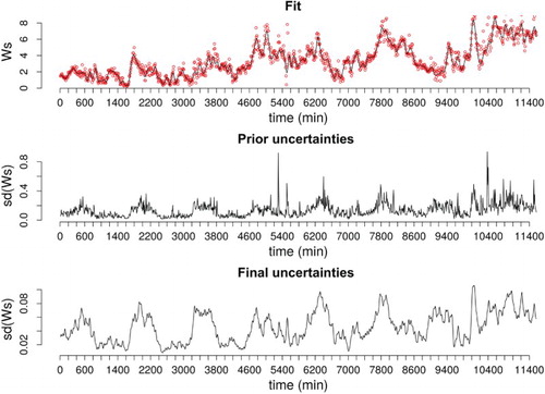
Table 1. Systematic sensor errors.

Parameter	Units	Set point	Error
Wind speed	m/s	0–5
Wind speed	m/s
Wind direction	degrees	0–360
Temperatures		30
Ventilation rates		60

Table 2. Considered parameters and relative prior distributions.

Num	Parameter	Type	Units	Initial estimate	Distribution	ID
1	Wind velocity	Multidimensional	m/s
2	Wind direction	Multidimensional	degrees
3	Ambient temperature	Multidimensional
4	Basement temperature	Multidimensional
5	Kitchen temperature	Multidimensional
6	Lobby temperature	Multidimensional
7	Bedroom 2 temperature	Multidimensional
8	Attic temperature	Multidimensional
9	Mech. vent. air temperature	Multidimensional
10	Mech. vent. inflow rate	Univariate		60	N(60, 1.75)
11	Mech. vent. outflow rate bathroom	Univariate		30	N(30, 0.88)
12	Mech. vent. outflow rate bedroom 1	Univariate		30	N(30, 0.88)
13	Lobby external door crack width	Univariate	mm	1
14	Lobby external door crack length	Univariate	m	2.4
15	Living room south window crack width	Univariate	mm	1
16	Living room south window crack length	Univariate	m	7.6
17	Living room west window crack width	Univariate	mm	1
18	Living room west window crack length	Univariate	m	2
19	Bedroom 1 window crack width	Univariate	mm	1
20	Bedroom 1 window crack length	Univariate	m	2
21	Bathroom window crack width	Univariate	mm	1
22	Bathroom window crack length	Univariate	m	2
23	Bedroom 2 window crack width	Univariate	mm	1
24	Bedroom 2 window crack length	Univariate	m	2
25	Kitchen window crack width	Univariate	mm	1
26	Kitchen window crack length	Univariate	m	2
27	Living-kitchen door crack width	Univariate	mm	2
28	Living-kitchen door crack length	Univariate	m	1
29	Living-lobby door crack width	Univariate	mm	2
30	Living-lobby door crack length	Univariate	m	1
31	Corridor-bedroom 2 door crack width	Univariate	mm	2
32	Corridor-bedroom 2 door crack length	Univariate	m	1
33	Living-basement crack width	Univariate	mm	2
34	Living-basement crack length	Univariate	m	1
35	Living-attic crack width	Univariate	mm	2
36	Living-attic crack length	Univariate	m	1
37	Pressure coefficient	Univariate	–	0.7
38	Pressure coefficient	Univariate	–	0.525
39	Pressure coefficient	Univariate	–	0.35
40	Pressure coefficient	Univariate	–	−0.075
41	Pressure coefficient	Univariate	–	−0.5
42	Pressure coefficient	Univariate	–	−0.45
43	Pressure coefficient	Univariate	–	−0.4
44	Pressure coefficient	Univariate	–	−0.3
45	Pressure coefficient	Univariate	–	−0.2
46	Pressure coefficient	Univariate	–	−0.3
47	Pressure coefficient	Univariate	–	−0.4
48	Pressure coefficient	Univariate	–	−0.450
49	Pressure coefficient	Univariate	–	−0.5
50	Pressure coefficient	Univariate	–	−0.075
51	Pressure coefficient	Univariate	–	−0.35
52	Pressure coefficient	Univariate	–	−0.053
101	Living room heater split	Univariate	–	0.7
102	Bedroom 1 room heater split	Univariate	–	0.7
103	Bathroom heater split	Univariate	–	0.7

Note: For pressure coefficients: (1) the angle is referred to the normal direction to the surface, and (2) they are repeated four times (once for each boundary node considered: NORTH, EAST, SOUTH and WEST).

Figure 4. Elementary effect representation in the coordinate system defined by PCA.

Figure 5. Main effects ( indexes) from the Morris Method for .

Table 3. First-order () and total effects () from the Sobol methods for .

Parameter
	0.42	0.46
	0.08	0.16
	0.00	0.00
	0.09	0.08
	0.02	0.02
LIF	0.25	0.31

Figure 6. Comparison between model predictions (black) and observed temperatures (red) (in colour online).

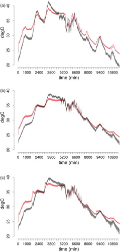
Table 4. Correlation between residuals and ROLBS heating sequences.

Parameter	Living room	Bedroom 1	Bathroom
ROLBS in living room	0.38	0.41	0.42
ROLBS in bedroom 1	0.38	0.41	0.42
ROLBS in bathroom	0.37	0.42	0.51

Figure 7. Comparison between prior (red crosses: quartiles, red dots: averages, blue dots: initial values) and posterior (boxplot) parameter distributions, for MIF. The samples have been normalized between 0 and 1 (in colour online).

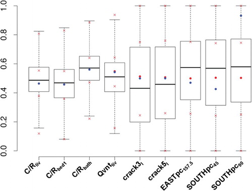
Table 5. Posterior estimates and 95% confidence intervals.

Parameter	Units	Posterior estimate	95% CI
	–	0.72	0.53	0.90
	–	0.71	0.50	0.90
	–	0.71	0.52	0.90
		59.4	54	61.2
	m	1.91	0.85	3.12
	m	1.93	0.87	3.14
	–	−0.20	−0.84	0.32
	–	−0.04	−0.56	0.40
	–	−0.36	−0.97	0.16

Table 6. First-order () and total effects () from the Sobol method relative to .

Parameter
	0.06	0.08
	0.20	0.39
	0.00	0.00
	0.08	0.12
	0.04	0.07
LIF	0.37	0.49

Figure 8. Comparison between prior (red crosses: quartiles, red dots: averages, blue dots: initial values) and posterior (boxplot) parameter distributions for LIF. The samples have been normalized between 0 and 1 (in colour online).

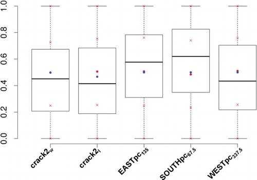
Figure 9. trend along parameter posterior variation ranges.

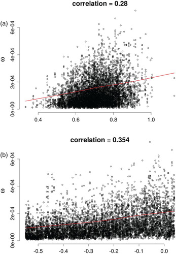
Figure 10. FS results by considering constant uncertainties for multidimensional variables.