Influence of error terms in Bayesian calibration of energy system models

Figures & data

Table 1. List of uncertain parameters in the calibration framework and selected prior probability distributions.

Parameter	Parameter description	Prior probability distribution
θ	Model (calibration) parameters	Normal (μ, σ)
λη	Precision parameter for model emulator	Gamma (10, 10)
λb	Precision parameter for model bias	Gamma (10, 0.3)
λe	Precision parameter for measurement error	Gamma (10, 0.03)
λen	Precision parameter for numerical error	Gamma (10, 0.001)
βη	Correlation strength parameter for model emulator	Beta (1, 0.5)
βb	Correlation strength parameter for model bias	Beta (1, 0.4)

Figure 1. Photos showing the Architecture Studio building (left) and the energy supply system cabinet with the heat pump on the bottom and the buffer tank on the top.

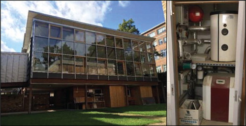
Figure 2. Schematic of the heat pump model in cooling mode with the corresponding input and output parameters. Uncertain parameters selected as calibration parameters are in italic.

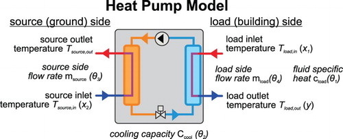
Figure 3. Measured field data and simulated computer data for the three data sets A, B and C showing the different temperature ranges and trends of each data set across the two dimension of load (upper plots) and source inlet temperature (lower plots).

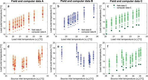
Figure 4. Results for predictive simulations for the emulator (a, d, g), the whole model term (b, e, h) and the model bias function (c, f, i) for data sets A, B and C over the load inlet temperatures (x₁).

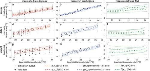
Figure 5. Results for predictive simulations for the emulator (a, d, g), the whole model term (b, e, h) and the model bias function (c, f, i) for data sets A, B and C over the source inlet temperatures (x₂).

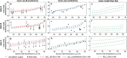
Figure 6. Prior and posterior probability distributions shown as boxplots for the reciprocal of the precision hyper-parameter λ_b and the correlation hyper-parameters (β_b1 refers to x₁, i.e. load side flow rate, β_b2 refers to x₂, i.e. source side flow rate) of the model bias for the three investigated data sets A, B and C. The centre line represents the median of the posteriors, boxes cover the interquartile range and whiskers include approx. 99% of the obtained posterior samples. The dashed line indicates the magnitude of the prior median value. Please note the parameter values do not represent the absolute value of the error term, as they are inferred from the normalized model data.

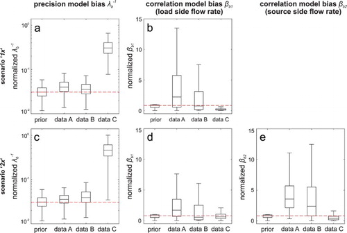
Figure 7. Prior and posterior distribution for the reciprocal of the random error λ_e and numerical error λ_en for different data sets on logarithmic scales. The centre line represents the median of the posteriors, boxes cover the interquartile range and whiskers include approx. 99% of the obtained posterior samples. The dashed line indicates the magnitude of the prior median value. Please note the parameter values do not represent the absolute value of the error term, as they are inferred from the normalized model data.

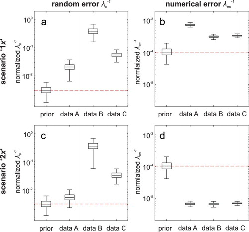
Figure 8. Prior and posterior distributions as boxplots for the four calibration parameters θ for different data sets. The centre line represents the median of the posteriors, boxes cover the interquartile range and whiskers include approx. 99% of the obtained posterior samples. The dashed line indicates the magnitude of the prior mode value.

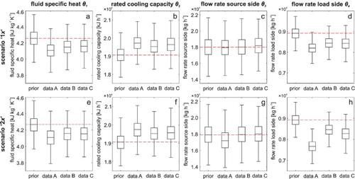
Figure 9. Posterior distributions of θ₁, θ₂, θ₄, λ_e⁻¹ and β_b for data sets A, B and C under scenario ‘1x’ for different priors on λ_b (GAM(10, 0.03), GAM(10, 0.1), GAM(10, 0.3), GAM(10, 1), GAM(10, 2.5) corresponding to an amount of variation in y caused by the model bias of ∼0.3%, ∼1%, ∼3%, ∼10% and ∼25%. The base case (∼3%) is indicated in bold. Resulting posteriors for θ₃ are not shown as this parameter is unidentifiable as well, and does not show any changes.

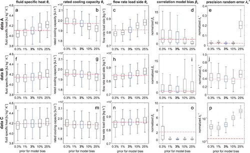
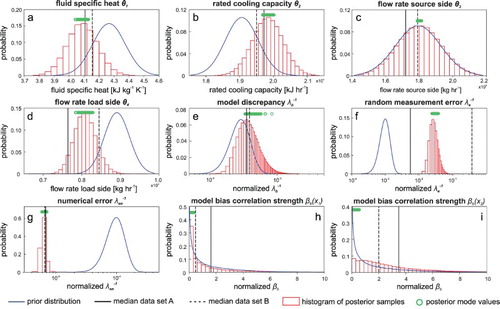
Figure 10. Prior distributions and combined histogram plots of all posterior samples from 199 converged calibration runs with 2000 samples each, inferred from the evaluation of the random data sets. The circles indicate the posterior median values of the individual 199 posterior sample sets, while the vertical solid and dashed lines indicate the posterior medians of data A and B, respectively. Note the logarithmic scale on the x-axes for the inverse of the model bias λ_b⁻¹, measurement error λ_e⁻¹ and numerical error λ_en⁻¹.