Figures & data
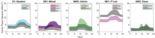
Figure 1. Plug load profiles (a) monitored demand and (b) typical profile assumed for simulation (O'Brien, Abdelalim, and Gunay Citation2018).
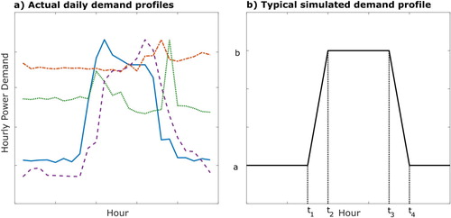
Figure 2. Sample demand profiles (a) may be generated from the action of a warping function (b) on an aligned amplitude function (c).
Figure 3. William Gates Building, Western side.

Figure 4. William Gates building, floor plan.
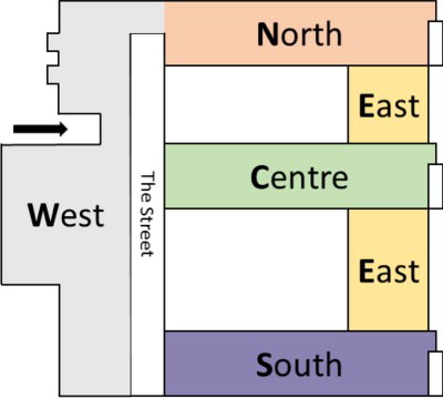
Table 1. William Gates building, spatial zone use types.
Figure 5. Daily monitored plug loads for 1 year for 10 different spatial zones showing the 90% confidence limits of demand for weekdays (red) and weekends (blue) (note variable scale on y-axis).
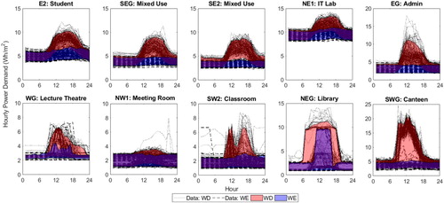
Figure 6. Amplitude principal components PCY 1–5, showing the impact of adding each PCY to the mean function (shown in black) using a positive (dashed) or negative (dotted) score.
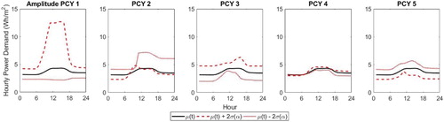
Figure 7. Phase principal components PCX 1–5, showing the impact of adding each PCX to the mean function (shown in black) using a positive (dashed) or negative (dotted) score.
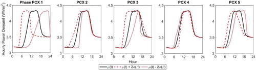
Figure 8. Scree plots showing the proportion of variability in the data accounted for by each PC for phase and amplitude.
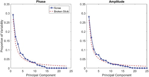
Figure 9. Impact of increasing the number of PCs included in the summation on the re-generation of the original data; with 1–5 PCs the base load is too low, but by 18 PCs the agreement is good.
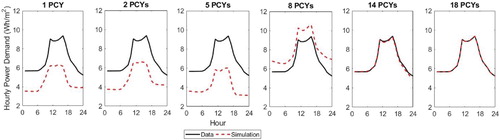
Table 2. PCY scores used for reconstitution of sample illustrated in Figure .
Figure 10. Scores for PCY 1 for 365 days' demand for each of 10 spatial zones; each point is the score for one day's data.
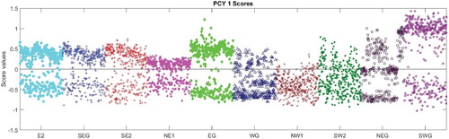
Figure 11. Scores for PCX 1 for 365 days' demand for each of 10 spatial zones; each point is the score for one day's data.
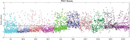
Figure 12. Amplitude scores (PCY 1) from Figure re-plotted by day of the week; weekend scores are noticeably lower for the majority of zones.
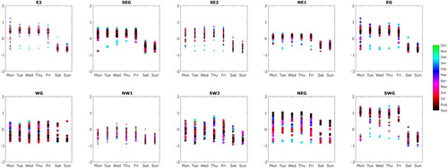
Figure 13. Phase scores (PCX 1) from Figure re-plotted by day of the week; weekend scores show a wider spread for the majority of zones.
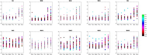
Figure 14. Scores for weekday (term 1) amplitude PCYs 1, primarily affecting load range, and 8, primarily affecting base load; an increase in score value in PCY 1 gives rise to an increasing load range, whereas a decrease in value in PCY 8 gives an increase in base load.

Figure 15. Scores for Zone SWG for amplitude PCs PCY 1/2, illustrating the non-normal scores distribution.
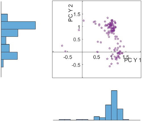
Figure 16. Sample scores for Zone SWG for amplitude PCs PCY 1/2, illustrating the fit achieved by using a Gaussian copula.
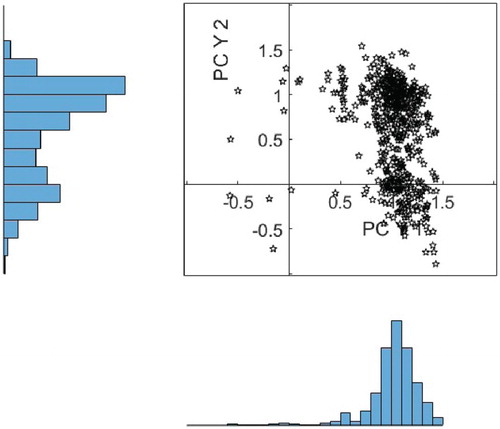
Figure 17. Sample profiles, term-time weekday; 90% confidence limits for 1000 samples generated by sampling from a Gaussian copula fitted to the score distributions (blue), compared against the training data (red) for 10 spatial zones.
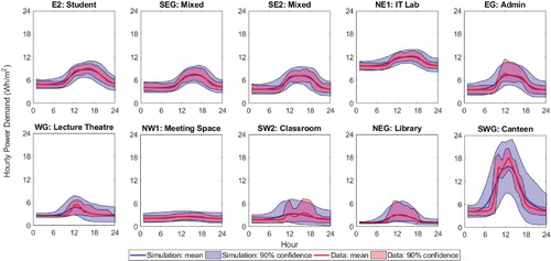
Figure 18. Base load for 1000 stochastic samples (Sim) compared against the training data for 10 spatial zones (term-time weekday).
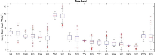
Figure 19. Daily total demand for 1000 stochastic samples (Sim) compared against the training data for 10 spatial zones (term-time weekday).
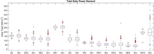
Figure 20. Peak load and timing of the peak for 1000 stochastic samples (Simulation) compared against the term-time weekday training data for 10 spatial zones (Data).
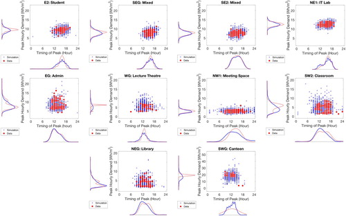
Figure 21. Comparison of amplitude scores for PCY1 and PCY8 generated for new spatial zones by mapping monitored data to the set of PCs derived from the training data, compared against scores for training zones with similar space-use type.
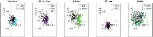
Figure 22. Comparison of monitored data for new spatial zones (grey) against monitored data for training zones with similar space-use type (90% confidence limit shown).