Figures & data
Figure 1. Barriers to adoption of large-scale BEM analysis. Marjorie Schott, National Renewable Energy Laboratory.
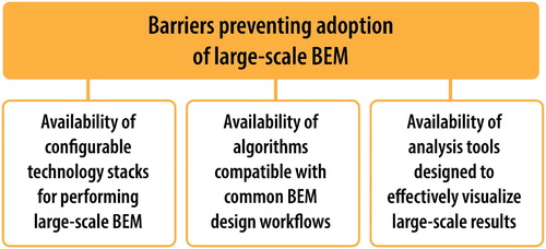
Figure 2. OSAF and Docker Swarm cluster architecture diagram. Marjorie Schott, National Renewable Energy Laboratory.
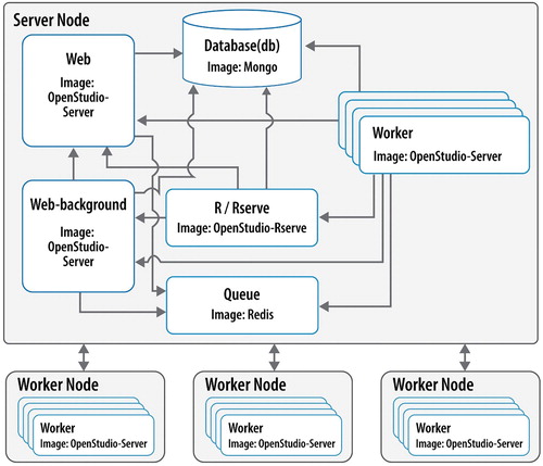
Figure 3. Deployment options of OSAF (laptop vs. local vs. cloud). Note that AWS stands for Amazon Web Services. Marjorie Schott, National Renewable Energy Laboratory.
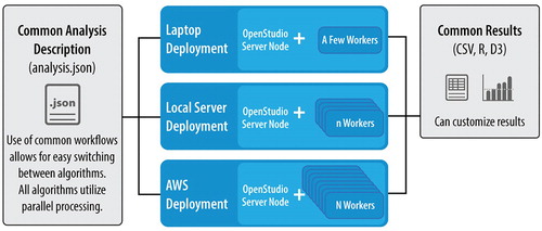
Figure 4. The OpenStudio Analysis (OSA) simulation process in OSAF (note that GUI stands for graphical user interface and OSW stands for OpenStudio Workflow). Marjorie Schott, National Renewable Energy Laboratory.
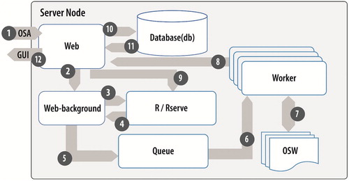
Figure 5. Example of an OpenStudio Analysis (OSA) problem formulation JSON.
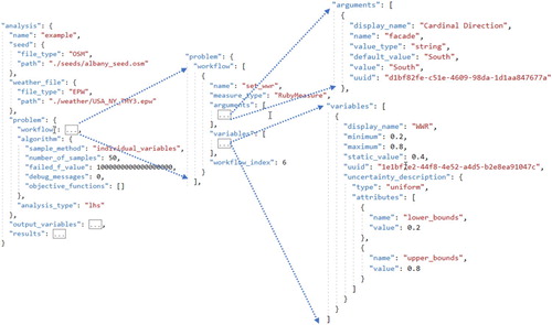
Figure 6. Example of defining a Measure variable in the Parametric Analysis Tool graphical user interface.
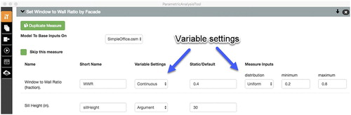
Figure 7. Example of changing algorithm type in the Parametric Analysis Tool graphical user interface.
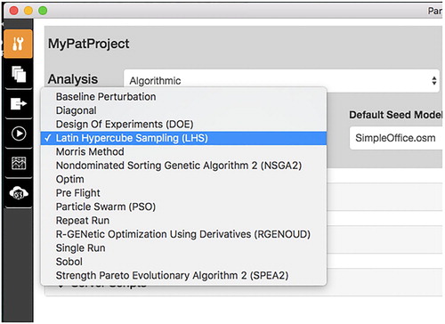
Figure 8. Example of an Interactive Parallel Coordinate Plot.
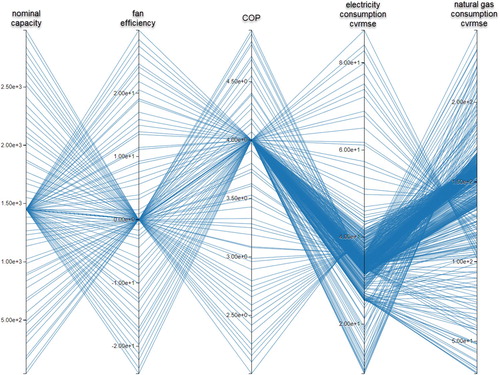
Figure 9. Interactive XY plot with Pareto frontier of annual total energy (gigajoules) vs. envelope cost (dollars).
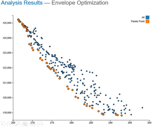
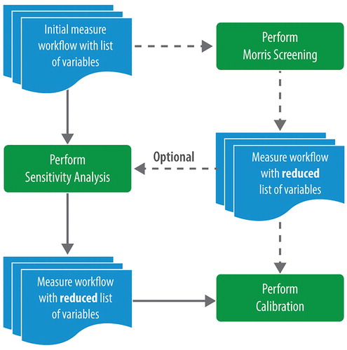
Figure 10. Algorithm switching for calibration problems. After performing a sensitivity analysis, a Morris screening, or both, inconsequential variables are removed, and algorithms are changed to optimization simply by changing the OSA JSON.