AixLib: an open-source Modelica library for compound building energy systems from component to district level with automated quality management

Figures & data

Figure 1. AixLib package structure comprising twelve packages.

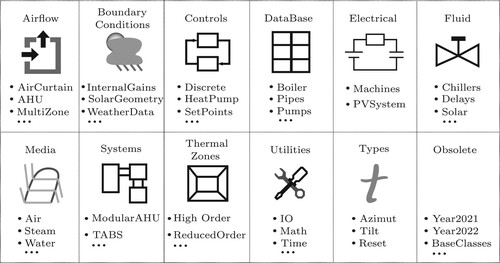
Figure 2. Structure of a building performance simulation. Connections with input/output causality contain arrows. Thermal and electrical connectors are depicted using squares. Fluid ports for water and air are bidirectional in Modelica. Nevertheless, we indicate the design direction (inflow / outflow).

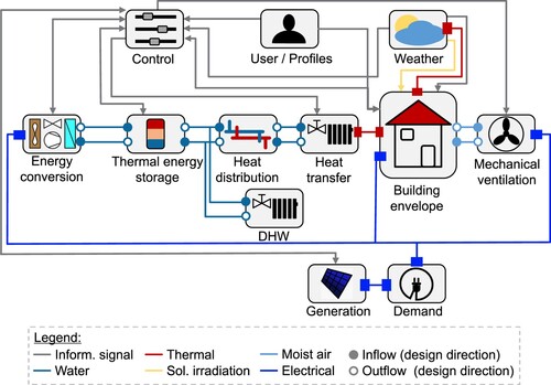
Figure 3. The seven stages of AixLib's continuous integration.

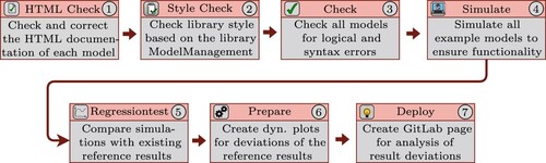
Table 1. Associated tools using or based on the AixLib library.

Toolname	Generative	Automation & Postprocessing
TEASER${}^{\mathrm{a}}$	X
uesgraphs${}^{\mathrm{b}}$	X
bim2sim${}^{\mathrm{c}}$	X
ebcpy${}^{\mathrm{d}}$		X
AixCaliBuHa${}^{\mathrm{e}}$		X

${}^{\mathrm{a}}$https://github.com/RWTH-EBC/TEASER

${}^{\mathrm{b}}$https://github.com/RWTH-EBC/uesgraphs

${}^{\mathrm{c}}$https://github.com/BIM2SIM/bim2sim

${}^{\mathrm{d}}$https://github.com/RWTH-EBC/ebcpy

${}^{\mathrm{e}}$https://github.com/RWTH-EBC/AixCaliBuHA

Figure 4. The air-handling unit use case with Modelica-specific icons. The system boundaries (e.g. exhaust air, outdoor air, etc.) set predefined input values for the system like the inlet temperatures and pressures. The controller and weather data are external boundary conditions which are connected via signal busses. The building model and the air-handling unit are connected using fluid ports.

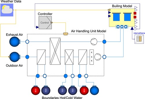
Figure 5. Exemplary results for the air-handling unit use case.

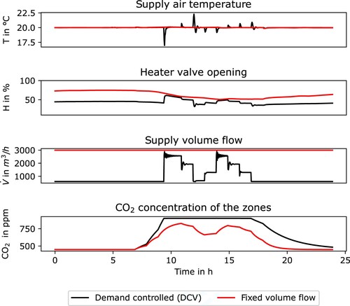
Figure 6. Coupled building energy system layout of use case 2 with a hydronic heat pump system.

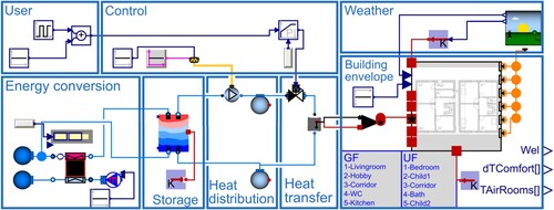
Table 2. Factors and levels of the full factorial design in use case 2.

Factor	V in l	k	$T_{\mathrm{I}}$ in s
Min	100	0.01	10
Max	1900	0.2	300
Number of levels	10	5	5

Figure 7. Room temperatures for rooms with different temperature setpoints for four combinations (a-d) of storage volume $V_{\mathrm{Sto}}$ and PI parameters ($k_{\mathrm{HP}}$ and $T_{\mathrm{I},\mathrm{HP}}$).

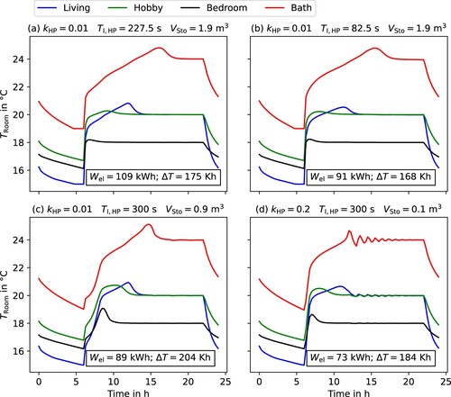
Figure 8. GIS illustration of Shamrockpark district for third use case.

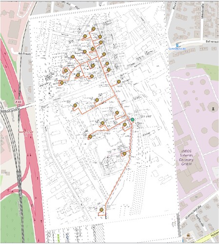
Figure 9. Modelica graphics view on northern part of Shamrockpark district. For better visualization the southern part is not illustrated. However, the same modelling principles apply.

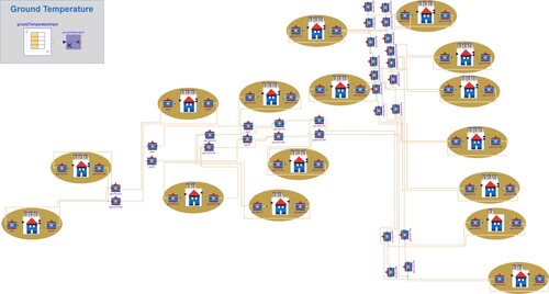
Figure 10. Annual performance simulation of thermal demands of the whole Shamrockpark district in Germany.

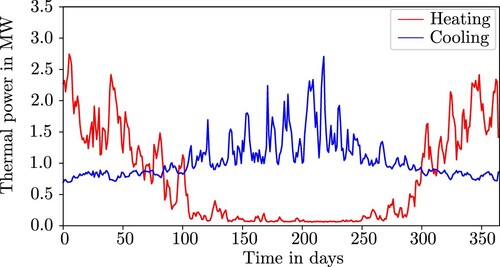
Figure 11. The energy supply structure to meet heating and cooling demands.

Table 3. Computation time, simulation time, number of model equations, number of state events, and the real-time factor for the three use cases. Use case 2 includes the four cases highlighted in Figure 7.

Use case	Computation time	Simulation time	Number of state events	Number of equations	Real-time factor
1	58.2 s	7 d	51	11456	10390
2a	18.1 s	2 d	25	25136	9547
2b	19.2 s	2 d	25	25136	9016
2c	22.4 s	2 d	45	25136	7711
2d	21.6 s	2 d	23	25136	7992
3	6.3 h	365 d	45402	49168	1395

Table 4. Excerpt from research projects succesfully applying AixLib models.

		Relevant components								Scale			Building type
Name	Description/aim	HP	B	Ch	AHU	TES	CTES	Bui	HN	dis	BES	C	R	NR	Ref. no.	Rel. citat.
AGENT	Agent-based model predictive control							x			x			x	03ET1495	Storek et al. (2022)
BIM2Sim and BIM2Praxis	Semi-automatic creation of dynamic simulation models based on BIM	x	x	x	x	x	x	x			x			x	03ET1562	Jansen et al. (2021)
Digital Twin	Digital twin for heat pump	x										x	x		03EN1022	Vering et al. (2022)
dECOnhealth	Demand controlled ventilation in hospitals				x			x			x			x	03ET1568	Rätz et al. (2020)
EESchwimm	Analysis of energy efficiency measures for swimming facilities using dynamic simulation		x		x	x		x			x			x	03EN1004	Kühn et al. (2022)
EnModuS	Influence of reduced air change rates in retail buildings on indoor air quality and energy consumption				x			x			x			x	03ET1502	Finkbeiner et al. (2021)
FUBIC: All-electricity	Demand calculation and digital twin for optimal control of laboratory and office building	x			x	x	x	x			x			x	03EN3026	Henn et al. (2022)
LivingRoadmap	Development of an energy supply concept with model predictive control based on a modernization roadmap		x	x				x	x	x				x	03ET1352	Wetter et al. (2019)
Moisture Recovery Systems	Potential analysis of enthalpy exchangers in air-handling units				x			x				x		x	25EWN	Kremer et al. (2019)
OOM4ABDO	Topology detection of sensor networks and fault detection in air-handling units	x	x			x					x			x	03SBE0006	Stinner et al. (2022)
TransUrban.NRW	Digital twin of four city districts for design and control optimization	x		x		x		x	x	x	x		x	x	03EWR020	Blacha et al. (2019)
Urban Energy Lab 4.0	Realistic emulation of future city concepts in a highly interconnected infrastructure	x						x			x		x	x	EFRE-0500029	Streblow (2022)
ZUGABE	Future hydraulic networks and their standardization in buildings	x	x	x	x	x	x	x			x	x	x	x	03ET1298	Kümpel et al. (2022)

Notes: The research projects differ regarding their aim, the components assessed, and the level of detail. The following abbreviations apply: HP:=Heat pump, B:=Boiler,Ch:=Chiller, AHU:=Air-handling unit, TES:=Thermal energy storage, CTES:=Cold thermal energy storage, Bui:=Building, HN:=Thermal network dis:=District, BES:=Building energy system, C:=Component, R:=Residential, NR:=Non-residential, Ref.No.=Reference Number of funding source, Rel. citat.:=Relevant citation.

Storek, T., F. Wüllhorst, Koßlerm Silas, M. Baranski, A. Kümpel, and D. Müller. 2022. “A Virtual Test Bed for Evaluating Advanced Building Automation Algorithms.” In 17th International Conference of the International Building Performance Simulation Association (BS 2021). Red Hook, NY: Curran Associates Inc. https://www.ebc.eonerc.rwth-aachen.de/go/id/dncb/file/843202.

 Google Scholar

Jansen, D., E. Fichter, V. E. Richter, A. Barz, J. Brunkhorst, M. Dahncke, P. Jahangiri, et al. 2021. “BIM2SIM – Development of Semi-automated Methods for the Generation of Simulation Models Using Building Information Modeling.” In Proceedings of Building Simulation 2021: 17th Conference of IBPSA.

 Google Scholar

Vering, C., S. Borges, D. Coakley, H. Krützfeldt, P. Mehrfeld, and D. Müller. 2022. “Digital Twin Design with On-Line Calibration for hvac Systems in Buildings.” In 17th International Conference of the International Building Performance Simulation Association (BS 2021). Red Hook, NY: Curran Associates Inc.

 Google Scholar

Rätz, M., P. Kalliomäki, P. Mathis, H. Koskela, and D. Müller. 2020. “Analyzing the Energy-Saving Potential of Demand-Controlled Ventilation in Hospitals Via Dynamic Building Simulations.” In 16th International Conference on Indoor Air Quality and Climate, edited by International Society of Indoor Air Quality and Climate. New York: Red Hook. https://publications.rwth-aachen.de/record/805261.

 Google Scholar

Kühn, L., A. Poensgen, V. Dannapfel, T. Osterhage, and D. Müller. 2022. “Indoor Swimming Pools: A Dynamic Simulation Model for Energy Analyses.” In Proceedings of BauSIM 2022.

 Google Scholar

Finkbeiner, K., M. Kremer, M. Rätz, X. Ying, P. Mathis, and D. Mueller. 2021. “Effect of Reduced Air Change Rates on Indoor Air Quality and Air Conditioning Energy.” In Building Simulation 2021 Conference. https://doi.org/10.18154/RWTH-2021-09080.

 Google Scholar

Henn, S., J. Richarz, L. Maier, X. Ying, T. Osterhage, P. Mehrfeld, and D. Müller. 2022. “Influences of Usage Intensity and Weather on Optimal Building Energy System Design with Multiple Storage Options.” Energy and Buildings 270:112222. https://doi.org/10.1016/j.enbuild.2022.112222.

 Web of Science ®Google Scholar

Müller, D., C. Treeck, R. Streblow, J. Frisch, M. Mans, P. Remmen, E. Spinnräker, and D. Koschwitz. “Entwicklung eines energieversorgungskonzeptes mit modellbasierter prädiktiver regelung anhand einer living roadmap am beispiel des forschungszentrums jülich : Schlussbericht : Eneff:stadt, eneff:campus: Livingroadmap, Entwicklung eines Energieversorgungskonzeptes mit modellbasierter prädiktiver Regelung anhand einer Living Roadmap am Beispiel des Forschungszentrums Jülich. https://doi.org/10.2314/KXP:168713295X.

 Google Scholar

Stinner, F., B. Llopis-Mengual, T. Storek, A. Kümpel, and D. Müller. 2022. “Comparative Study of Supervised Algorithms for Topology Detection of Sensor Networks in Building Energy Systems.” Automation in Construction 138:104248. https://doi.org/10.1016/j.autcon.2022.104248.

 Web of Science ®Google Scholar

Blacha, T., M. Mans, P. Remmen, and D. Müller. 2019. “Dynamic Simulation of Bidirectional Low-Temperature Networks – A Case Study to Facilitate the Integration of Renewable Energies.” In Proceedings of Building Simulation 2019: 16th Conference of IBPSA, Rome, Italy. https://doi.org/10.26868/25222708.2019.210670.

 Google Scholar

Streblow, R. 2022. “Rwth aachen – Urban Energy Lab 4.0.” https://www.uel4-0.de/Home/.

 Google Scholar

Kümpel, A., J. Teichmann, P. Mathis, and D. Müller. 2022. “Modular Hydronic Subsystem Models for Testing and Improving Control Algorithms of Air-handling Units.” Journal of Building Engineering 53:104439. https://doi.org/10.1016/j.jobe.2022.104439.

 Web of Science ®Google Scholar

Data availability statement

The data that support the findings of this study are available from the corresponding author, Laura Maier, upon reasonable request.