Insight into the avidity–affinity relationship of the bivalent, pH-dependent interaction between IgG and FcRn

Figures & data

Figure 1. Assay orientations to investigate the interaction between a monovalent and bivalent-binding partner. (a) The monovalent partner as solute analyte = FcRn. (b) The bivalent partner as solute analyte = IgG. Illustrations are created with BioRender.com.

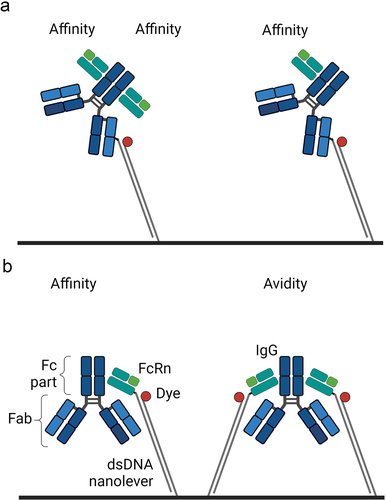
Table 1. The relationship between assay orientation, ligand density, and resulting binding modes. IgG = bivalent binder, FcRn = monovalent binder.

Assay orientation	A	B
Ligand is immobilized	IgG (bivalent)	FcRn (monovalent)
Analyte in solution	FcRn (monovalent)	IgG (bivalent)
Ligand density	Binding mode(s)
Low	Affinity	Affinity
Medium^a	Affinity	Affinity/Avidity
High^b	Affinity	Avidity

^aContributions of affinity and avidity modes should be of similar magnitude for good fit quality.

^bMeasurement artifacts (rebinding, mass transport limitations) are likely to occur at high ligand densities, which is why measurements have to be interpreted with care.

Figure 2. Kinetic analysis of immobilized human FcRn and a human IgG1 (mAb1) in solution at pH 6.0 utilizing a medium FcRn density on a switchSENSE biosensor chip. (a) shows the schematic assay configuration allowing affinity and avidity to occur simultaneously. mAb1 was injected in five different concentrations as two-fold dilution series with a highest concentration of 300 nM for hIgg1 Fc WT (b) and 60 nM for hIgg1 Fc YTE (c). Each plot (b,c) shows the measured raw data (gray) and the global fit analysis as solid lines (blue fading). The sensorgram display a monophasic association phase and biphasic dissociation phase reflecting affinity and avidity binding mode. The determined kinetic parameters are described in Table 2. Illustration a is created with BioRender.com.

Table 2. Summary of the affinity and avidity measurements of immobilized human FcRn and an mAb1 Fc variants in solution using a switchSENSE biosensor chip having a medium ligand density. The kinetic rate parameters are determined from analyzing the sensorgrams shown in Figure 2. The k_ON, k_OFF and K_D values are results from a global fit analysis ± fitting error.

Sample		Affinity		Avidity
	kON (x10^6 M^−1s^−1)	kOFF,AFFINITY (x10^−2 s^−1)	KD,AFFINITY (nM)	kOFF,AVIDITY (x10^−2 s^−1)	KD,AVIDITY (nM)
hIgG1 Fc WT	7.53 ± 0.38	34.2 ± 1.50	45.4 ± 3.0	4.70 ± 0.30	6.24 ± 0.51
hIgG1 Fc YTE	8.42 ± 0.15	2.60 ± 0.06	3.09 ± 0.09	0.25 ± 0.01	0.29 ± 0.01

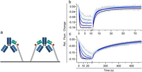
Table 2. Summary of the affinity and avidity measurements of immobilized human FcRn and an mAb1 Fc variants in solution using a switchSENSE biosensor chip having a medium ligand density. The kinetic rate parameters are determined from analyzing the sensorgrams shown in Figure 2. The k_ON, k_OFF and K_D values are results from a global fit analysis ± fitting error.

Sample		Affinity		Avidity
	kON (x10^6 M^−1s^−1)	kOFF,AFFINITY (x10^−2 s^−1)	KD,AFFINITY (nM)	kOFF,AVIDITY (x10^−2 s^−1)	KD,AVIDITY (nM)
hIgG1 Fc WT	7.53 ± 0.38	34.2 ± 1.50	45.4 ± 3.0	4.70 ± 0.30	6.24 ± 0.51
hIgG1 Fc YTE	8.42 ± 0.15	2.60 ± 0.06	3.09 ± 0.09	0.25 ± 0.01	0.29 ± 0.01

Figure 3. Kinetic analysis of human FcRn immobilized and a human IgG1 (mAb1) Fc YTE mutant in solution at nine different pH values on switchSENSE biosensor chip. mAb1 Fc YTE was injected in five different concentration as two-fold dilution series with a highest concentration of (a) 60 nM at pH 5.8, (b) 60 nM at pH 6.0, (c) 100 nM at pH 6.2, (d) 150 nM at pH 6.4, (e) 200 nM at pH 6.6, (f) 300 nM at pH 6.8, (g) 400 nM at pH 7.0, (h) 800 nM at pH 7.2 and (i) 800 nM at pH 7.4. Note that the x axis for each sensorgram (a – i) has a different time scale. Each plot (a – i) shows the measured raw data (grey) and the global fit analysis as solid lines (blue fading). For (a – h) the dissociation phase is biphasic characterized by two different dissociation rate constants reflecting the affinity (1:1) and the avidity (2:1) binding mode. The interaction displays a biphasic dissociation curve reflecting affinity and avidity binding where one or two hFcrn are engaged with one mAb1 Fc YTE. The dissociation of mAb1 Fc YTE and hFcrn at pH 7.4 (I) is described by a monophasic fit model reflecting the affinity binding mode (1:1) where one hFcrn is engaged with one mAb1 Fc YTE. Panel (J) shows the applied, exemplary biphasic fit model for FcRn with mAb1 Fc YTE mutant injecting 300 nM at pH 6.0. The adequacy of the fit model is confirmed by the minimal residuals, indicating no significant deviation. The association phase occurred to be monophasic while the dissociation phase is biphasic. The overall dissociation curve is superposition of two exponential time-courses, namely the affinity binding mode (fast dissociation) and the avidity binding mode (slow dissociation). The measured data is shown in blue and the fit in black solid lines, whereas the two deconvoluted exponential time-courses are shown in grey as dashed lines. The contribution of fast and slow dissociation to the overall signal change is shown as Amplitude A_fast or A_slow. The determined kinetic parameters are described in Table 3.

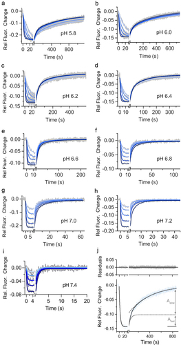
Table 3. Summary of the affinity and avidity measurements of immobilized human FcRn and mAb1 Fc YTE mutant as solute using a switchSENSE biosensor chip having a medium ligand density. The kinetic rate parameters are determined from analyzing the sensorgrams shown in Figure 3. The k_ON, k_OFF and K_D values are results from a global fit analysis ± fitting error.

hIgG1 Fc YTE		Affinity		Avidity
pH	kON (x10^6 M^−1s^−1)	kOFF,AFFINITY (x10^−2 s^−1)	KD,AFFINITY (nM)	kOFF,AVIDITY (x10^−2 s^−1)	KD,AVIDITY (nM)
5.8	7.58 ± 0.11	2.15 ± 0.03	2.84 ± 0.06	0.17 ± 0.01	0.23 + 0.01
6.0	8.42 ± 0.15	2.60 ± 0.06	3.09 ± 0.09	0.25 ± 0.01	0.29 ± 0.01
6.2	6.42 ± 0.17	3.39 ± 0.07	5.28 ± 0.18	0.45 ± 0.01	0.70 ± 0.03
6.4	6.14 ± 0.14	6.57 ± 0.12	10.7 ± 0.31	0.94 ± 0.01	1.53 ± 0.04
6.6	9.23 ± 0.42	12.8 ± 0.46	13.9 ± 0.80	2.05 ± 0.12	2.22 ± 0.17
6.8	6.20 ± 0.31	26.3 ± 1.62	42.4 ± 3.38	4.83 ± 0.35	7.79 ± 0.69
7.0	4.69 ± 0.21	44.1 ± 1.92	94.0 ± 5.86	7.51 ± 0.37	16.0 ± 1.06
7.2	3.81 ± 0.18	90.0 ± 0.54	236 ± 18.0	17.6 ± 0.71	46.2 ± 2.87
7.4	2.41 ± 0.45	119 ± 6.00	494 ± 95.5	NA	NA

Figure 4. Schematic depiction of a bivalent analyte (IgG) interacting with a monovalent ligand (FcRn). State 0 shows the free state of monovalent FcRn (immobilized) and bivalent IgG (in solution). The transition from State 0 to State 1 illustrates that the bivalent analyte associates with one binding site on FcRn (k_ON1 and k_OFF1). in its subsequent transition to State 2 the IgG concurrently binds via its second binding site to another FcRn, which is in close proximity to the first one, thereby forming a bivalent complex. The avidity occurs accordingly to the absolute and relative contributions of the individual on- and off-rates of the transitions 0 ↔ 1 and 1 ↔ 2. The dynamic dissociation and re-association of one to two binding sites, the transition 2 ↔ 1 ↔ 2 (k_ON^app. and k_OFF^app.), is crucially important for the effective off-rate and hence for the avidity. Typically, it is impossible to differentiate between singly bound and doubly bound states within the measurement signal. As a result, only the ‘observable’ kinetic rates (k_ON^obs. and k_OFF^obs.) between the free and any type of bound state are measured. The illustration is created with BioRender.com.

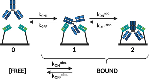
Figure 5. Rate scale plot of FcRn (ligand) and mAb1 YTE variant (solute) at a pH from 5.8 to 7.4. The plot allows the comprehensive comparison of multiple kinetic rate parameters obtained from several kinetic experiments/sensorgrams at one glance. The upper plot shows the association rate (k_ON) while the lower plot shows the dissociation rate (k_OFF) as logarithmic scale. Each kinetic rate parameter pair is connected via a vertical line where its length or else the distance of the two data points gives insights about the binding strength of the measured interaction. The proximity of the data points corresponds to a weaker interaction, or in other words, an increase in the dissociation constant K_D. The data points are shown as mean ± SD* (*smaller than the data points, thus not visible). To obtain an inflection point the affinity dissociation rates (k_OFF,AFFINITY) are fitted by a Four Parameter Logistic (4PL) fit shown in gray (Equation (6)(6) $\mathit{y}=\mathit{d}+\frac{\mathit{a}-\mathit{d}}{1+{\left(\frac{x}{c}\right)}^{\mathit{b}}}$(6) ) resulting in a transition at pH 7.2 (Figure S11).

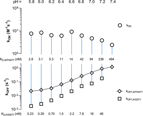
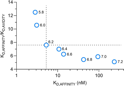
Figure 6. Avidity-to-affinity relationship of FcRn and mAb1 YTE variant from pH 5.8 to 7.2. The ratio of the K_D values (K_D,AFFINITY/K_D,AVIDITY), referred to as avidity enhancement factor increases from neutral to acidic pH. The higher the binding strength (affinity) the more its contribution to the overall avidity enhancement. Weak affinities occurring at pH 6.4 to 7.4 only show a minor contribution to the avidity effect while strong affinities from pH 5.8 to 6.2 show higher contribution. A transition point is pH 6.2, indicated by the dashed lines. The data points are shown as mean ± SD* (*smaller than the data points, thus not visible).