Emergence of informative higher scales in biological systems: a computational toolkit for optimal prediction and control

Figures & data

Figure 1. Comparing micro to macro. (a) A biological micro-scale, here a set of ion channels opening and closing, which makes up the membrane potential. (b) A causal model, and abstraction of the workings of the system at the micro-scale, is created by the modeler or experimenter (generally via interventions). This causal model might represent the openings and closings of channels, or the interactions of other molecular interactions, and may have a very high number of parameters. (c) Biological systems often have available macro-scales which are some dimension reduction of the micro-scale. An example might be the membrane potential of a cell. Often these biological macro-scales have interventions that manipulate them directly, such as current injection to change the variables or states can only be manipulated at the macro-scale. (d) A macro-scale causal model is an abstraction, wherein each variable or element might represent that state of the macro-scale and the effects of changes of those states, like how increases the membrane potential might lead to further changes in neighboring cells.

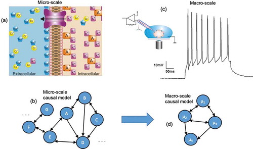
Figure 2. Measuring information in the causal structure of a network. (a) The entropy of a random walker’s next movement while standing on node A reflects the noise intrinsic to A’s outputs (note that this calculation requires normalizing the total weight of each node’s output to sum to 1.0). (b) <W_i ^out > is the distribution of weight across the network (found by averaging across nodes in the network). (c) The EI is a function of the determinism minus the degeneracy of the network, which allows for the characterization of network architecture.

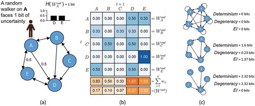
Figure 3. GRN coarse-graining. (a) The GRN as a Boolean network. Note Isl1 has further projections into the larger cardiac regulatory network, but since these are not represented, it is instead given a self-loop as is traditional in Boolean analysis for nodes without outputs. (b) The expanded state-space wherein each node is a binary string of exogen_canWnt_II, Foxc1_2, Fgf8, CanWnt, Isl1. (c) Using a greedy algorithm that groups different sets of nodes together the possible partitions can be explored in a search for only those groupings that improve the EI. (d) Once the appropriate groupings are identified the network can be represented in its dimensionally-reduced format. Here the macro-nodes μ₁ and μ₂ are constructed in the simplest way possible, as a coarse-grain.

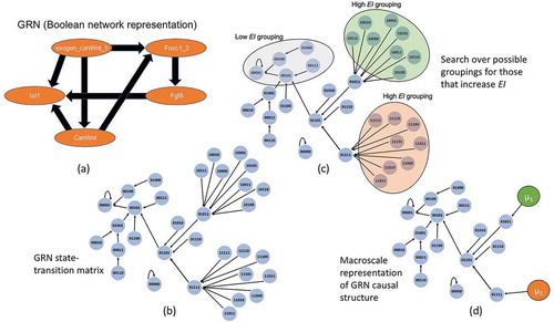
Figure 4. Macro-scale of Saccharomyces cerevisiae GRN. (Left) The largest component of the Saccharomyces cerevisiae gene regulatory state-space, derived from the Boolean network GRN representation. (Right) The same network but grouped into a macro-scale, found via the greedy algorithm outlined in [48]. There is a ~ 66% reduction in total states and an increase in the network’s EI. Green nodes represent macro-nodes in the new network.

Klein B , Hoel E . The emergence of informative higher scales in complex networks. Complexity. 2020;2020:1–12.

 Web of Science ®Google Scholar