Biologically-inspired neuronal adaptation improves learning in neural networks

Figures & data

Figure 1. An example of neuron activity during the free and clamped phases with adjusted adaptation. For visual clarity, only one representative neuron from the top layer is shown. The time steps for free and clamped phases are 120, and teaching signals are given after 12 steps. The adjusted adaptation steps are 20. After 120 steps at the clamped phase, additional 20 steps for the adaptation are applied using Eq. 8(8) ${\hat{x}}_{adp,t+1}=\left(1-c\right){\hat{x}}_{adp,t}+c\ast \underset{\ast }{\overset{\vee }{x}}$(8) .

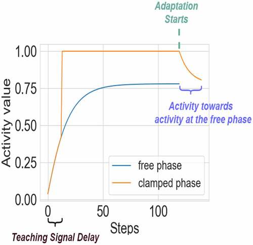
Figure 2. The learning curves for the models (parameters: 782-50-10) with the adjusted adaptation (MLP-ADP) and without the adjusted adaptation (MLP) on MNIST.

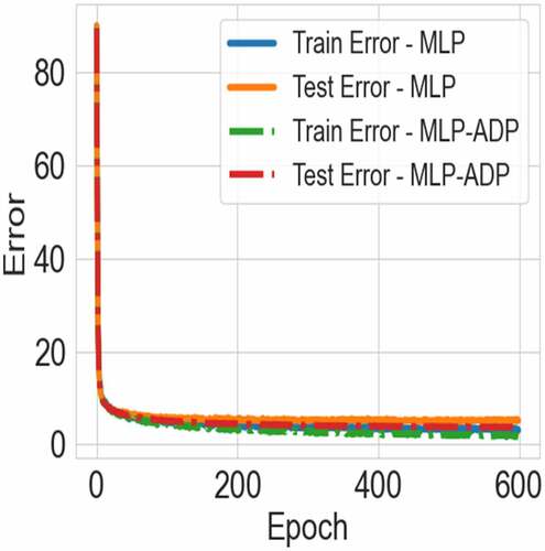
Figure 3. The learning curves for the models with the adjusted adaptation (CNN-ADP) and without the adjusted adaptation (CNN) on CIFAR-10.

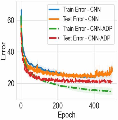
Table 1. Training results on MNIST and CIFAR-10 with EP and the adaptation/no adaptation. For MNIST, we trained MLP with CHL. For CIFAR-10, we trained CNNs with EP. For laterl1, the lateral connections are only in the hidden layer. For lateral2, the lateral connections are in both hidden and output layers. We trained each network six times to calculate average and ±the standard deviation. Numbers in bold denote smallest test error.

	No Adaptation (error %)		Adaptation (error %)
	Test	Train	Test	Train
MNIST (MLP)
784-6-10	17.29 ± 1.78	16.11 ± 1.77	11.93 ± 0.84	9.45 ± 1.06
784-50-10	4.63 ± 0.19	2.71 ± 0.22	3.56 ± 0.1	1.62 ± 0.09
784-50-10; lateral 1	4.56 ± 0.30	2.54 ± 0.24	3.82 ± 0.13	1.76 ± 0.12
784-50-10; lateral 2	4.88 ± 0.33	2.81 ± 0.36	3.86 ± 0.18	1.84 ± 0.11
784-1000-10	1.98 ± 0.04	0.00 ± 0.00	1.77 ± 0.06	0.01 ± 0.00
784-1000-10; lateral 1	1.85 ± 0.05	0.00 ± 0.00	1.78 ± 0.06	0.01 ± 0.00
784-1000-10; lateral 2	1.83 ± 0.06	0.00 ± 0.00	1.81 ± 0.07	0.01 ± 0.00
CIFAR10 (CNN)
256-512	22.46 ± 0.59	22.88 ± 1.71	19.51 ± 0.6	14.70 ± 2.31

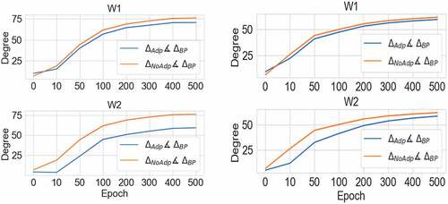
Figure 4. Mean angle between weight gradients calculated using BP and CHL (left: 6 neurons a hidden layer, right: 12 neurons in a hidden layer). Blue line shows the angle calculated for CHL with adaptation, and orange for CHL without adaptation. “W1” means the gradients for the weights between the input and hidden layers, and “W2” means the gradients for the weights between the hidden and output layers. The angle between the gradients with the adaptation and BP is denoted as ∆Adp∡∆BP . The angle between the gradients without the adaptation and BP is denoted as ∆NoAdp∡∆BP . Note that the blue line is consistently closer to 0, which demonstrates that CHL with adaptation provides weights updates more similar to BP gradients.