Figures & data
FIGURE 1 Locations (stars) at which American shad were sampled in the Santee–Cooper River basin and the Pee Dee River.
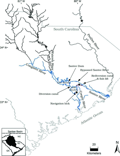
TABLE 1 Summary information for American shad sampling in the Santee–Cooper and Pee Dee River basins. Fish were sampled over the course of the spawning run except for the Pee Dee River; N = the sample size.
TABLE 2 Probability values for tests of genic differentiation among sampling sites for American shad in the Santee–Cooper basin based on 10 microsatellite loci. All comparisons were nonsignificant following sequential Bonferroni correction (Rice Citation1989).
TABLE 3 Pairwise comparisons of D EST estimates for American shad sampling locations in the Santee–Cooper basin. The values above the diagonal are D EST values based on 10 microsatellite loci; those below the diagonal are the corresponding P-values. All comparisons were nonsignificant following sequential Bonferroni correction (Rice Citation1989).
FIGURE 2 Values of ΔK averaged across three replicate simulations versus the simulated number of groups (K) observed in the data. The simulation results indicate that the most plausible value for K represented by American shad from the Santee–Cooper basin is 2, as evidenced by the distinct reduction in ΔK from K = 2 to K = 3. Note, however, that the proportion of sampled individuals to each group was symmetrical for all K = 2–8, which is an indication of no population structure (Evanno et al. Citation2005).
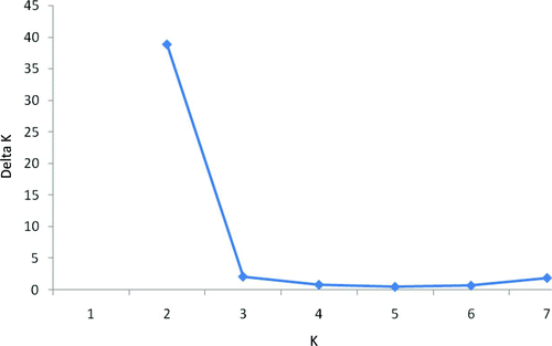
TABLE 4 Comparison of genetic diversity and the fixation index between wild and hatchery samples of American shad from the Santee–Cooper basin at various microsatellite loci. We tested for homogeneity in the average number of alleles (NA), observed heterozygosity (HO ), expected heterozygosity (HE ), and the fixation index (F) between a random sample of the 2009 broodstock (Santee River, hatchery; n = 83) and wild fish collected from throughout the Santee–Cooper system during the course of the study (n = 283). All comparisons between average values were nonsignificant.
TABLE 5 Comparison of genetic diversity and the fixation index between American shad from the Santee–Cooper (n = 283) and Pee Dee River basins (n = 43) at various microsatellite loci. The estimates of allelic richness are based on 43 individuals. All comparisons between average values are nonsignificant. See for additional information.
FIGURE 3 Percent parentage assignment success versus number of loci for simulated American shad parents and progeny (red curves), along with type II errors with and without data on mating history. The simulated numbers of broodstock males and females were (A) 314 and 255 and (B) 5,000 and 5,000. The simulations assumed a 3% genotyping error rate and that all broodstock were genotyped for all loci. Type II errors were estimated by performing parentage analysis on simulated wild progeny and hatchery broodstock. The inferred mating history allowed 25 males and 25 females to spawn together and was similar to hatchery conditions.
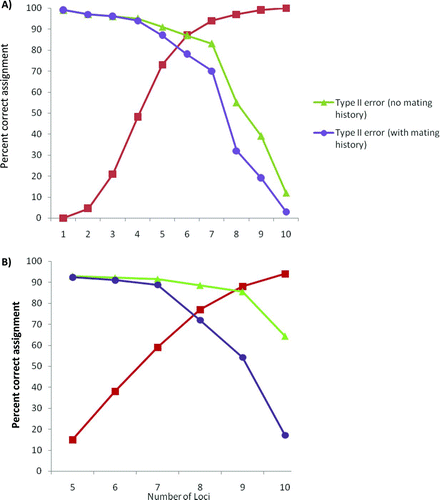
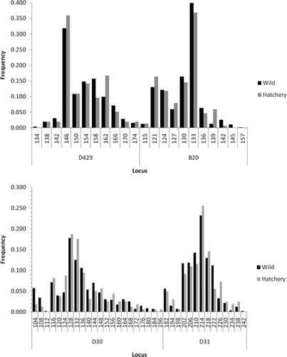
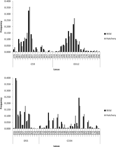
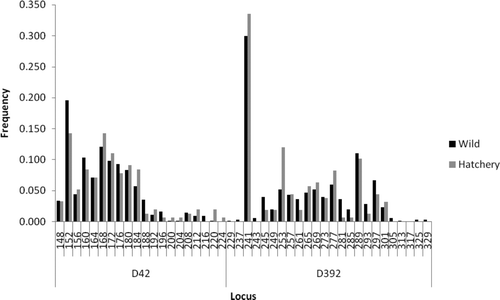
FIGURE A1 Comparison of allele frequencies at various microsatellite loci between hatchery and wild American shad from the Santee–Cooper River basin.