Figures & data
TABLE 1 Average zooplankton abundance in several North Carolina coastal river systems as determined by various studies.
FIGURE 1 Locations of the sampling stations and delineation of the three sampling areas in the lower Roanoke River and Albemarle Sound, North Carolina.
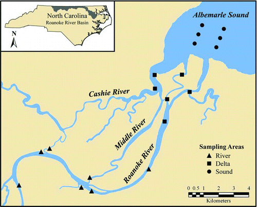
TABLE 2 Prey and American shad stocking densities from Johnson and Dropkin (Citation1995) and Riley et al. (Citation2012). The stocking densities given on a per-liter basis represent the values used in the experiments. Those converted to a per-cubic-meter basis allow comparison with the abundances in this study. To determine the ratio of prey to larvae, the prey density was divided by that of American shad.
TABLE 3 Average monthly values (means ± SDs) for environmental variables collected in March–June 2008 and 2009 in the lower Roanoke River and Albemarle Sound.
TABLE 4 Comparison between the values (means ± SDs) of environmental parameters in 2008 and 2009 in the lower Roanoke River and Albemarle Sound.
TABLE 5 Mean values of environmental variables in the three sampling areas in the lower Roanoke River and Albemarle Sound. Means with common letters are not significantly different at the 0.5 level according to the Ryan–Einot–Gabriel–Welch procedure.
FIGURE 2 Weekly zooplankton abundance in (a) River, (b) Delta, and (c) Sound in 2008 and 2009. Note the differences in the scale of the y-axis.
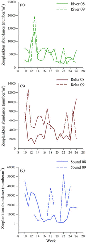
FIGURE 3 Monthly zooplankton composition in (a) River, (b) Delta, and (c) Sound in 2008 and (d) River, (e) Delta, and (f) Sound in 2009. Abbreviations are as follows: Cal = calanoid copepods, Cyc = cyclopoid copepods, Nauplii = copepod nauplii, Clad = cladocerans, and Rot = rotifers.
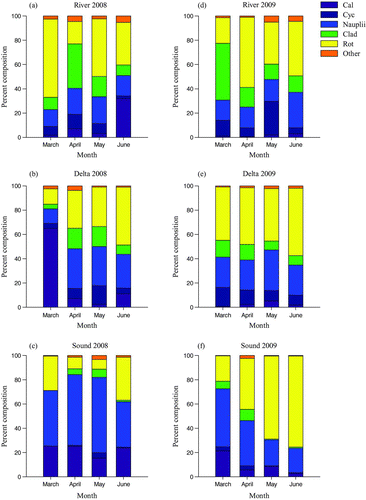
FIGURE 4 Nonmetric multidimensional scaling ordination plot illustrating the similarity among samples in respect to area for zooplankton samples collected in the Roanoke River and Albemarle Sound.
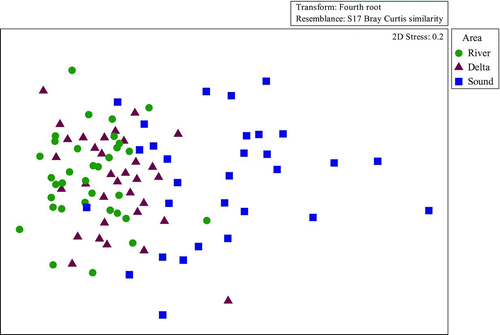
TABLE 6 SIMPER analysis evaluating the dissimilarity between areas identified as significantly different using ANOSIM. Abundances are fourth-root transformed. The average Bray–Curtis dissimilarity scores are listed as average dissimilarity. Diss/SD identifies how consistently taxa contribute to the dissimilarity. Asterisks identify discriminating taxa. The contribution percentage is the amount of dissimilarity that can be attributed to a taxon.
FIGURE 5 Mean weekly abundance of larval alewives, blueback herring, and hickory shad in (a) 2008 and (b) 2009 in the Roanoke River and Albemarle Sound. Note the differences in the scale of the y-axis.
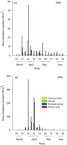
FIGURE 6 Frequency distributions of four alosine species based on notochord length. Note the differences in the scale of the y-axis.
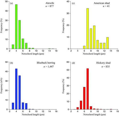
FIGURE 7 Mouth gape regression models for (a) alewives, (b) blueback herring, (c) American shad, and (d) hickory shad. The models were calculated with the mouth open at 90°. Note the differences in the scales of the both axes.
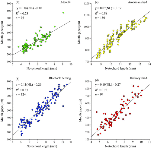
FIGURE 8 Body lengths and widths for the most common zooplankton taxa. Values are means ± SDs. The dashed lines represent the maximum prey size for larval alewives, blueback herring, and hickory shad at first feeding. The dotted lines represents the maximum prey size for larval American shad at first feeding.
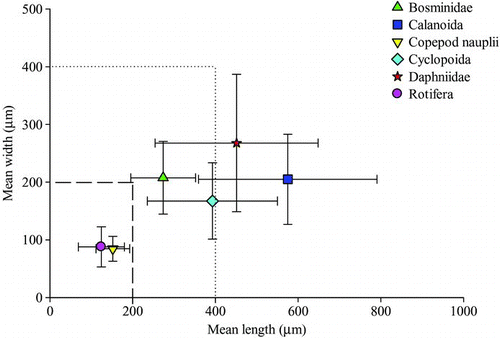
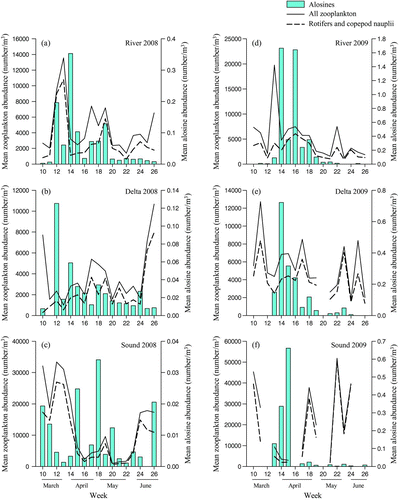
FIGURE 9 Zooplankton and larval alosine spatiotemporal overlap in (a) River in 2008, (b) Delta in 2008, (c) Sound in 2008, (d) River in 2009, (e) Delta in 2009, and (f) Sound in 2009. Note the differences in the scale of the y-axes (left and right).
