Socially-aware evaluation framework for transportation

Figures & data

Figure 1. Themes in the framework.

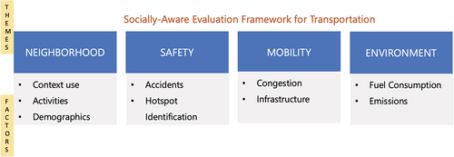
Figure 2. Indicators for each theme.

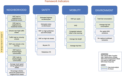
Figure 3. SAEF Indicators and their spatial levels.

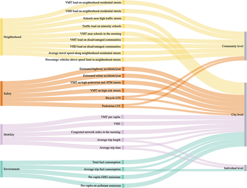
Figure 4. Mobiliti simulation framework.

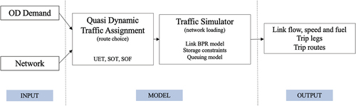
Figure 5. Bay area cities colored by per capita trips.

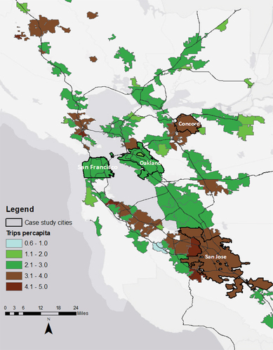
Table 1. Case study cities.

City	Area (sq.mile)	Population	Population density (person/sq.mile)	Trips per capita
San Jose	185	1,021,795	5,524	3.1
San Francisco	49	874,961	17,847	2.2
Oakland	58	425,097	7,333	2.7
Concord	31	129,183	4,105	3.5

Figure 6. Network typologies for Bay Area. Neighborhood residential streets constitute the highest share, followed by highways. Individual cities reflect similar partitioning.

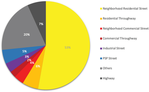
Figure 7. Network typologies for Oakland, San Jose, San Francisco, and Concord. Oakland has the highest percentage of highways, and Concord has the highest percentage of neighborhood residential streets.

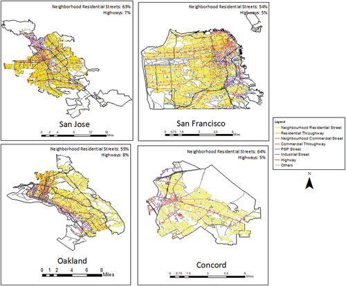
Table 2. Methods used to evaluate indicators.

Theme	Indicator	Method
Neighborhood	VMT load on neighborhood residential streets, VHD load on neighborhood residential streets	Section IV-B, IV-C1
	Schools near high traffic streets, Traffic load on minority schools, VMT near schools in the morning	Section IV-C1
	VMT load on disadvantaged communities, VHD load on disadvantaged communities	Section IV-C1
Safety	Estimated highway accidents/year	Section IV-C2
Mobility	VMT per capita, VHD, Congested network miles in the morning, Average trip length, Average trip time	Section IV-C3
Environment	Total fuel consumption, Average trip fuel consumption	Section IV-C3

Figure 8. Theme Neighborhood: Communities of Concern census tracts in the case study cities. Oakland has the highest percentage of population living in these census tracts and Concord the least.

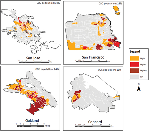
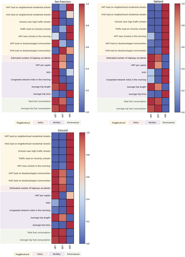
Figure 9. SAEF indicators for San Jose. Each metric is normalized to a scale between 0 and 1. Red and blue represent high and low, respectively. For instance, VHD indicator in the mobility theme is high for SOF and low for SOT

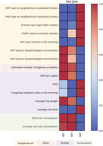
Figure 10. Theme Neighborhood: The figure illustrates the schools (blue circles) affected by high and medium traffic volume. Red links have an ADT greater than 50,000, and yellow links have ADT between 25,000 and 50,000. The number of impacted schools is higher with SOF routing.

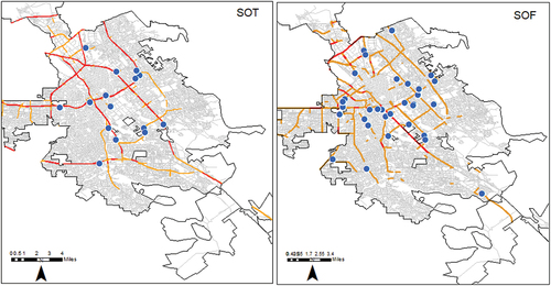
Figure 11. Theme Mobility: The figure shows the difference in VMT for SOT (left) and SOF (right) compared to baseline UET for San Jose. The red or green represents the increase or decrease in VMT, and the thickness represents the magnitude of the difference. Only highways and neighborhood residential streets are shown. It can be seen that SOF has shifted a significant amount of traffic from highways (broad green lines) to residential streets (thin red lines) in an attempt to reduce fuel consumption.

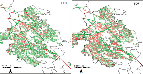
Figure 12. The figure compares SAEF metrics across cities for different route optimizations. The metrics are numbered from 1 to 15 on the chart. They are normalized with respect to the maximum values for a city so that the relative differences can be identified. For example, in San Jose, SOF has the highest values for metrics 1, 2, 3, 4, 5, 10, 11, and 13. In San Francisco, UET has the highest values for metrics 2, 3, 6, 8, 9, 10, 11, 14, and 15. Overall, the comparison reveals that UET performs worse for San Francisco whereas SOF performs worse for all other cities.

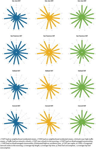
Table A1. SAEF indicator description.

Theme	Indicator	Description	Unit	Spatial level	Temporal level
Neighborhood	VMT load on neighborhood residential streets	It is calculated as the proportion of vehicle miles traveled on neighborhood residential streets to the proportion of the network miles in neighborhood residential streets. City streets need to be classified based on complete streets guidelines to identify neighborhood residential streets based on land use and transport functionalities. A load greater than 1 signifies a disproportionate impact.	Ratio	Community	Entire day/Peak hours
Neighborhood	VHD load on neighborhood residential streets	It is calculated as the proportion of vehicle hours of delay on neighborhood residential streets to the proportion of the network miles in neighborhood residential streets. City streets need to be classified based on complete streets guidelines to identify neighborhood residential streets based on land use and transport functionalities. A load greater than 1 signifies a disproportionate impact.	Ratio	Community	Entire day/Peak hours
Neighborhood	Schools near high traffic streets	Streets with Average Daily Traffic (ADT) greater than 50,000 and 25,000 are considered high-traffic streets and medium-traffic streets, respectively. All roads within 250 m of the school vicinity is considered for this analysis.	Number	City	Entire day
Neighborhood	Traffic load on minority schools	The traffic load on minority schools is calculated as the proportion of minority schools impacted by traffic to the proportion of minority schools in the city. Minority schools are identified based on the demographic characteristics of the children in the school.	Ratio	City	Entire day
Neighborhood	VMT near schools in the morning	Vehicle miles traveled in the 250 meter vicinity of schools. VMT is calculated for 7–8 am. This indicator helps in understanding the difference in traffic flow around schools for various routing strategies.	Miles	City	Peak hours
Neighborhood	VMT load on disadvantaged communities	It is calculated as the proportion of vehicle miles traveled on the streets in the disadvantaged communities to the proportion of the network miles in disadvantaged communities. Disadvantaged communities can be identified based on city’s definition.	Ratio	Community	Entire day
Neighborhood	VHD load on disadvantaged communities	It is calculated as the proportion of vehicle hours of delay on the streets in the disadvantaged communities to the proportion of the network miles in disadvantaged communities. Disadvantaged communities can be identified based on city’s definition.	Ratio	Community	Entire day
Neighborhood	Average travel speed along neighborhood residential streets	Average travel speed on neighborhood residential streets can be calculated for morning or evening peaks. This will give an estimate of how the traffic moves in neighborhoods.	Miles per hour	Community	Entire day/Peak hours
Neighborhood	Percentage vehicles above the speed limit in neighborhood streets	Percentage of vehicles traveling above the posted speed limit at different times of the day indicates how traffic flow affects the quality of life in neighborhoods.	Percentage	Community	Peak hours
Safety	Estimated highway accidents/year	Highway accidents estimated based on traffic volume and road geometry. Safety performance functions for highways can be used.	Number	City	Entire day
Safety	Estimated urban accidents/year	Urban accidents estimated from traffic volume, road geometry and other factors. Standard methods from the literature can be adopted.	Number	City	Entire day
Safety	VMT on high pedestrian and ATM streets	Vehicle miles traveled on streets with high Active Transportation Mode (ATM) users and pedestrians. It measures the multi modal safety of roads. Routing strategies that increases VMT on these roads hinders others active users of the road.	Miles	City	Entire day/Peak hours
Safety	VMT on high risk streets	High risk roads are roads with hot spots, steep slopes and sharp turns which can be dangerous when unknown drivers are routed through them.	Miles	City	Entire day/Peak hours
Mobility	Bicycle level of traffic stress	Bicycle Level of Traffic Stress (LTS) rating can be calculated for road segments based on the type of facility, traffic volume and speed. Standard methods from literature can be adopted for calculation.		City/Community	Peak hours
Mobility	Pedestrian level of traffic stress	Pedestrian LTS rating can be calculated for road segments based on the type of facility, traffic volume and speed. Standard methods from the literature can be adopted for calculation.		City/Community	Peak hours
Mobility	VMT per capita	Total miles traveled by all vehicles in the system divided by the city’s population.	Miles per capita	City	Entire day
Mobility	VHD	Total hours of delay incurred by all vehicles in the system. It is computed as the difference between the actual travel time and free flow travel time for all trips.	Hours	City	Entire day
Mobility	Congested network miles in the morning	Congested miles are roads with volume over capacity greater than or equal to 1 during morning hours. This measures the congested network for each routing strategy.	Miles	City	Peak hours
Mobility	Average trip length	Average length of all the trips that start or end in a city. It can be segregated into work and nonwork trips.	Miles	Individual/City	Entire day
Mobility	Average trip time	Average travel times for all the trips that start or end in a city. It can be segregated into work and nonwork trips .	Minutes	Individual/City	Entire day
Environment	Total fuel consumption	Total fuel consumption for all vehicles in a city.	Liters	City	Entire day
Environment	Average trip fuel consumption	Average fuel consumption for all trips that start or end in a city.	Liters	Individual/City	Entire day
Environment	Per capita GHG emissions	GHG emissions per person in a city. Methods to calculate emissions from vehicular traffic can be adopted from the literature.	CO2e	City	Entire day
Environment	Per capita air pollutant emissions	Air pollutant emissions per person in a city. Methods to calculate emissions from vehicular traffic can be adopted from the literature.	Micrograms per cubic meter	City	Entire day

Table A2. Functional road classes.

Functional Class	Definition
1	Allowing for high volume, maximum speed traffic movement
2	Allowing for high volume, high speed traffic movement
3	Providing a high volume of traffic movement
4	Providing for a high volume of traffic movement at moderate speeds between neighborhoods
5	Roads whose volume and traffic movement are below the level of any other functional class

Table A3. Network typologies for Bay Area.

Sl No	Street Type	Length (thousand miles)	Remarks
1	Neighborhood Residential Street	26	Neighborhood streets with adjoining residential land use
2	Residential Throughway	2.9	Throughway streets with adjoining residential land use
3	Neighborhood Commercial Street	1.8	Neighborhood streets with adjoining commercial land use
4	Commercial Throughway	1.1	Throughway streets with adjoining commercial land use
5	Industrial Street	1.7	Neighborhood or Throughway streets with adjoining industrial land use
6	PSP Street	2.5	Neighborhood or Throughway streets with adjoining public and semi public land use
7	Highway	3.4	Highways including ramps
8	Others	9.9	Includes streets with adjoining land use as green spaces, undeveloped land,parking lots, water bodies etc.

Table A4. SPF parameters for California highways.

Number of lanes	alpha	beta
1	−7.09	0.98
2	−7.09	0.98
3	−7.09	0.98
4	−5.78	0.82
5	−6.49	0.89
6	−6.49	0.89
7	−6.49	0.89
8	−10.75	1.24

Table A5. Summary of Results: SAEF for case study cities.

City Indicator	San Jose			San Francisco			Oakland			Concord
	UET	SOT	SOF	UET	SOT	SOF	UET	SOT	SOF	UET	SOT	SOF
VMT load on neighborhood residential streets	0.07	0.07	0.17	0.22	0.24	0.35	0.09	0.10	0.30	0.07	0.07	0.10
VHD load on neighborhood residential streets	0.01	0.01	0.06	0.14	0.05	0.10	0.01	0.01	0.09	0.01	0.01	0.02
Schools near high traffic streets	19	21	41	32	31	31	17	17	51	0	0	1
Traffic load on minority schools	1.66	1.93	2.09	1.96	2.03	2.30	0.86	0.86	1.30	0	0	2.55
VMT near schools in the morning	82,301	82,696	93,039	95,630	92,923	99,252	94,386	92,478	99,089	2,378	2,483	4,203
VMT load on disadvantaged communities	1.56	1.54	1.45	1.32	1.30	1.30	1.19	1.18	1.28	1.62	1.60	1.42
VHD load on disadvantaged communities	2.00	1.89	1.66	1.22	1.59	1.51	1.13	1.15	1.41	1.28	1.18	0.46
Estimated number of highway accidents	4,844	4,615	175	1,650	1,534	876	3,065	2,915	581	528	507	39
VMT per capita	18.57	18.35	16.78	11.22	11.08	10.63	23.57	22.94	20.25	17.74	17.65	17.71
VHD	10,665	5,682	21,857	16,947	5,919	10,366	9,298	4,873	18,268	578	382	1,399
Congested network miles in the morning	46.43	19.78	91.97	32.88	16.43	17.01	19.38	8.96	41.26	1.00	0.76	4.79
Average trip length	8.40	8.30	8.02	7.42	7.43	7.18	8.94	8.88	8.52	9.17	9.14	8.93
Average trip time	10.10	10.03	14.04	10.52	10.29	13.74	11.43	11.23	17.04	11.06	10.97	15.54
Total fuel consumption	2,883,657	2,871,752	1,828,504	995,748	979,577	816,895	1,441,556	1,418,620	872,783	328,744	327,188	240,779
Average trip fuel consumption	1.33	1.34	0.86	1.03	1.04	0.77	1.41	1.43	0.95	1.49	1.50	1.04

Figure 13. SAEF results for San Francisco, Oakland and Concord.