Figures & data
Figure 1. Extended possibility for the monitoring of food quality during various stages of the supply chain of a product.
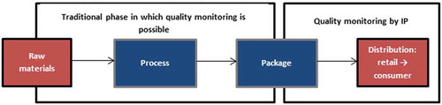
Figure 2. Schematic illustration of intelligent packaging (IP) with sensors that monitor environmental conditions, or quality attributes of the product related to overall food quality change. The environmental condition sensor can also be placed inside the package depending on the measured condition. Source: Adapted from Heising et al. (Citation2014b).
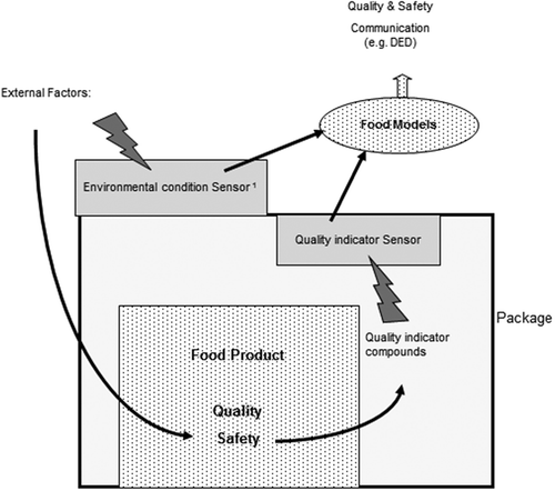
Figure 3. Overview of the use of intelligent packaging (IP) to communicate about its quality attributes. Although there are always reactions going on in foods, some quality attributes remain relatively constant for a long time. Whether or not a quality attribute changes after processing depends on both the food type and shelf life. For example, the quality attribute ‘nutritional value’ of fresh fish will not change much during its life cycle since the sensory changes happen much faster and are rate limiting for the shelf life of the product. Therefore, nutritional value is considered stable in fresh fish, although lipid oxidation can become important (rate limiting) in fish with a longer shelf life. Some quality attributes can be estimated well by consumers, e.g., the colour of bananas indicates their ripeness. In this case there is no need to monitor this quality attribute by an intelligent package. To monitor a quality attribute, product properties that can be measured in a non-destructive way in the package must give a good indication of the quality attribute. Source: Adapted from Heising et al. (Citation2014b).
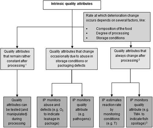
Figure 4. Conceptual model for using IP-DED in QCL to reduce waste.
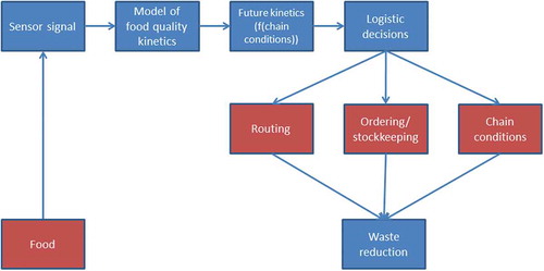
Figure 5. Simplified general supply chain used in this modelling approach.
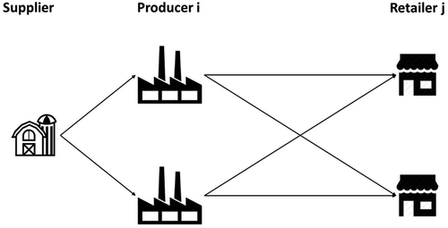
Table 1. Notation used in the model.
Table 2. Distribution of the quality levels of the initial food product supply for the different scenarios in fraction of the total supply.
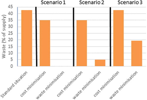
Figure 6. Waste percentages in the standard situation and after optimising the different scenarios.