Figures & data
Figure 1. Reference state (a) where the elastomer is unstretched and uncharged. A is the inner radius of the unstretched elastomer and B is the outer radius. Red circle denotes points at an arbitrary radius R. H is the initial thickness. Elastomer in (a) is biaxially prestretched and clamped at the outer and inner annulus (b). Inner and outer radius is constrained to a and b. The elastomer is then coated with complaint electrodes on both sides. Mechanical load F is applied in out of plane direction and a voltage of ϕ is applied as shown in (c). A section of (c) is enlarged in (d). Direction 1 is along the surface of Loudspeaker DEG towards the centre. Direction 2 is the hoops direction. s1 and s2 are the nominal stresses in 1 and 2 directions. λ1 and λ2 are stretches in 1 and 2 directions. θ is the angle the section makes with the horizontal plane. r and z are the coordinates of the deformed shape.
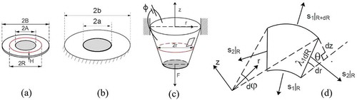
Figure 2. Sample of simulation result. Final deformed shape, λ1 and λ2, s1 and s2 and θ are plotted in (a), (b), (c) and (d) respectively. The simulation result is for, F = 1 and ϕ = 0 (solid line), ϕ = 0.2 (dashed line). A:B = 0.5 and λp = 2.
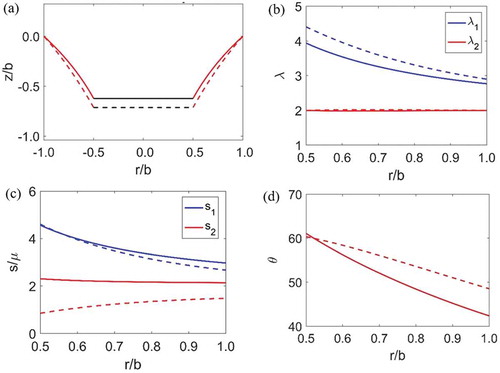
Figure 3. Force used is 0.5 (normalized with respect to b), prestretch used is 1.2 and A to B ratio is 0.25. Black, green, red and blue lines are for ϕ = 0, 0.15, 0.2 and 0.25 respectively. For (i) the Jlim used is, 120 and for (ii) it is 500. (iii) is re-created using the governing equations from [Citation9]. In that paper, the material model used is Neo-Hookean. Hence the results for a larger value of Jlim (ii) matches with theirs.
![Figure 3. Force used is 0.5 (normalized with respect to b), prestretch used is 1.2 and A to B ratio is 0.25. Black, green, red and blue lines are for ϕ = 0, 0.15, 0.2 and 0.25 respectively. For (i) the Jlim used is, 120 and for (ii) it is 500. (iii) is re-created using the governing equations from [Citation9]. In that paper, the material model used is Neo-Hookean. Hence the results for a larger value of Jlim (ii) matches with theirs.](/cms/asset/f692a91a-a877-4c58-8865-072af377a08e/tsnm_a_1421276_f0003_c.jpg)
Figure 4. Each black curve represents the state of loudspeaker DEG for a given force. An open circle represents the point of loss of tension. After loss of tension a new set of equations explained in section, ‘Post tension loss analysis’ are used. As the stretches are non-uniform, loss of tension and the instability in stretch occurs locally and progresses. This is represented by the dotted lines in the plot. The red curve represent rupture and the blue one represents electric breakdown. A:B = 0.5 and λp = 2.
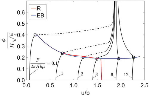
Figure 5. Voltage vs stretch at the inner ring and at the midway between inner and outer ring. Loss of tension and transition of stretches happens at different voltages. A:B = 0.5, λp = 2 and F = 1.
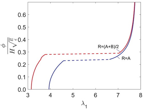
Figure 6. Final deformed shape, λ1 and λ2, s1 and s2 and θ are plotted in (a), (b), (c) and (d) respectively. The simulation result is for, F = 1 and ϕ = 0.25. Solid lines represent the simulation result using the new set of equations beyond loss of tension and dashed lines are the results without considering them. A:B = 0.5 and λp = 2.
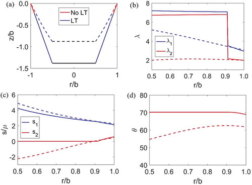
Figure 7. Progression of wrinkles. The simulation result is for, F = 1.5. At ϕ = 0.21, wrinkles appear near inner ring and at ϕ = 0.282, the entire membrane will be under loss of tension. A:B = 0.5 and λp = 2.
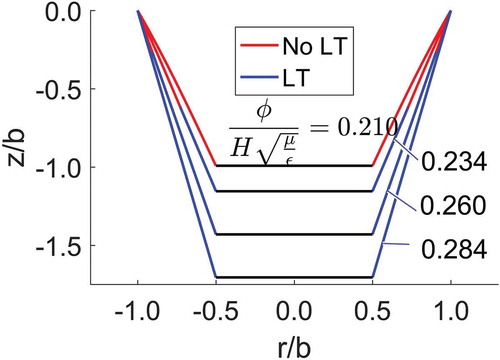
Table 1. Summary of tensile test data. is found nearly half of
. The average value of
from experiments is found to be 144.9. But for our analysis, we will still use the value of 120 from literature.
Figure 8. Comparison of deformed shape from theoretical prediction and experimental observation.
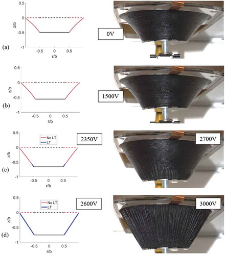
Figure 9. Voltage vs displacement plot. Blue cross indicates the point of electric breakdown.
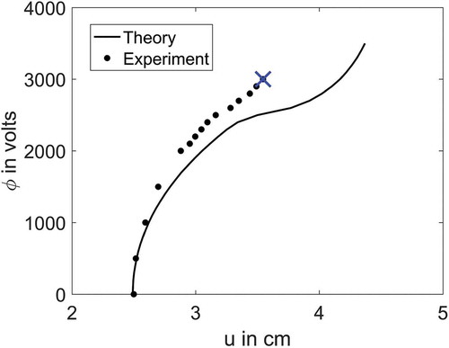
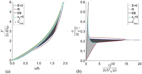
Figure 10. Operational boundaries of loudspeaker DEG. Green curve is the curve for zero electric field, red is the rupture curve, blue is the electric breakdown curve, black line is the minimum capacitance line and the cyan curve is the s2 = 0 line. The light grey area is the allowable states if we consider loss of tension as an operational limit. Dark grey area is the allowable states post tension loss. For force displacement diagram this region is narrow. A:B = 0.5 and λp = 2.
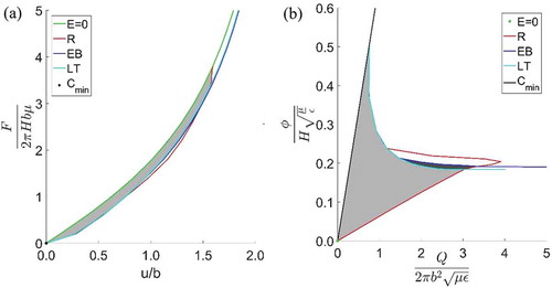
Figure 11. Non-dimensionalized energy vs A:B and λp. (a) is plotted with s2 = 0 as a limit – the DE is always operating in a non-wrinkled flat configuration and (b) exploits deformation post tension loss, with a small enhancement of energy of conversion in the region of low prestretch.
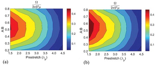
Figure 12. Specific energy vs A:B and λp. (a) is plotted with s2 = 0 as a limit – the DE is always operating in a non-wrinkled flat configuration and (b) exploits deformation post tension loss.
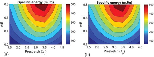
Figure 13. Operational boundaries of a hypothetical elastomer whose rupture limit, JR = 0.6 Jlim and electric breakdown strength, E√(ε/μ) = 7. A:B = 0.5 and λp = 2.