Figures & data

Figure 1. (a) preparation of sandwich-like MXene/CNT/CuNps films. (b) crop the sensor into a circle. (c) printing flexible circuits. (d) use conductive silver paste to combine sensors and flex circuits. (e) connect the sensor to the wire and cure it together with the composite material, then connect it to the data collector for work.
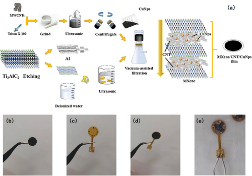
Figure 2. (a) Sensitivity test diagram of different thin film sensors. (b) MXene/CNT/CuNps stability test diagram. (c) Scanning electron microscopy of composite film under impact (Due to the small size of nano-copper, not marked in the figure). (d) Mechanism of sensor resistance change.
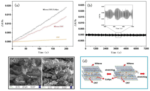
Figure 3. (a) one-dimensional sensor positioning principle.We can determine the impact location by the intersection of the two sensor functions. (b) two-dimensional sensor positioning principle.The impact point location is derived from the intersection of the three sensing radii.
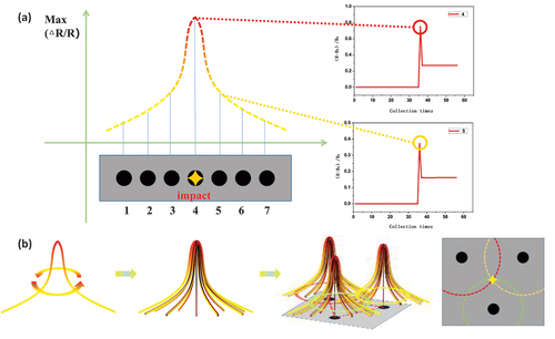
Figure 4. (a) Composite laminate layer 1 simulation. (b) Composite laminate layer 2 simulation.(c) Layer 1 and Layer 2 overlay simulation, which can be used to determine the optimal laying distance of the sensor. (d) Three-point sensor matrix array.
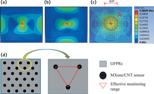
Figure 5. Principles of planar geometric analysis.
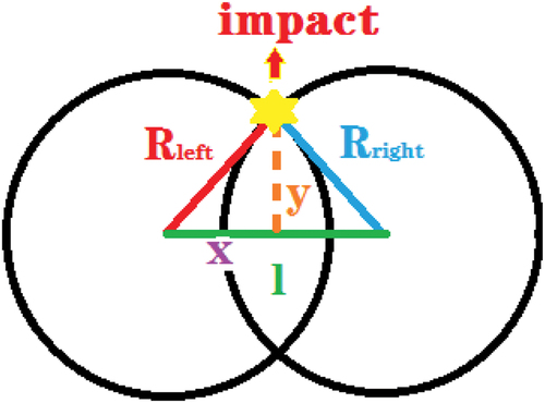
Figure 6. Schematic diagram of the weighted compensated positioning algorithm.
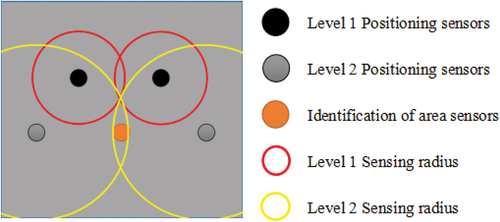
Figure 7. Schematic diagram of fabrication of composite laminates.
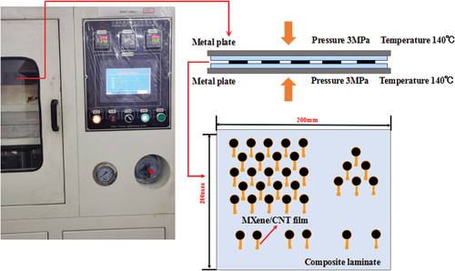
Figure 8. (a) sensor array area.Each sensor is assigned an independent number, and the data changes of each sensor in the experiment are recorded. (b) Low-velocity impact test setup.
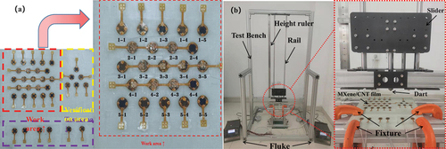
Figure 9. (a) select the 6 sensors with the largest resistance change from the 23 sensor data, and use different shapes and colors to represent the sensors with the largest resistance change rate.(b) compare the resistance response of each sensor after impact. It can be seen that the resistance change rate near the impact point is larger, and with the weighted compensation positioning algorithm, impact positioning monitoring can be performed.
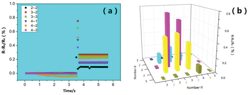
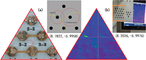
Figure 10. Input the maximum sensor resistance change rate indication after measurement.Through the weight function compensation positioning algorithm, the calculation result is(8.7822,-5.9958).
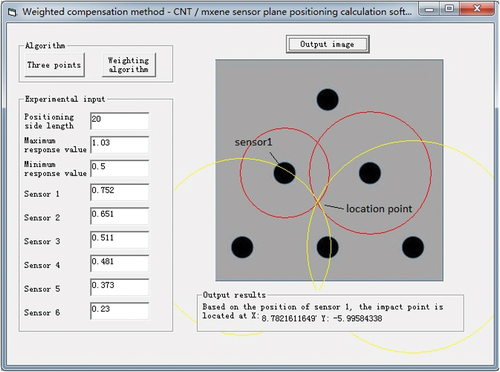
Figure 11. (a) the red circle is the positioning point obtained after calculation. (b) c-scan results of the impacted specimen.